Fitdistcp: fitting distributions using calibrating priors
fitdistcp is a free software package for fitting statistical distributions using calibrating priors. The goal of fitdistcp is to provide a way to fit distributions
in such a way that the fitted distributions make reliable (i.e., well calibrated) predictions. Standard methods for fitting distributions do not give reliable predictions, and so are of
questionable value for evaluating risk.
fitdistcp is available natively in both R and Python. The R version currently supports a wider range of models, and can be called from within Python (details below).
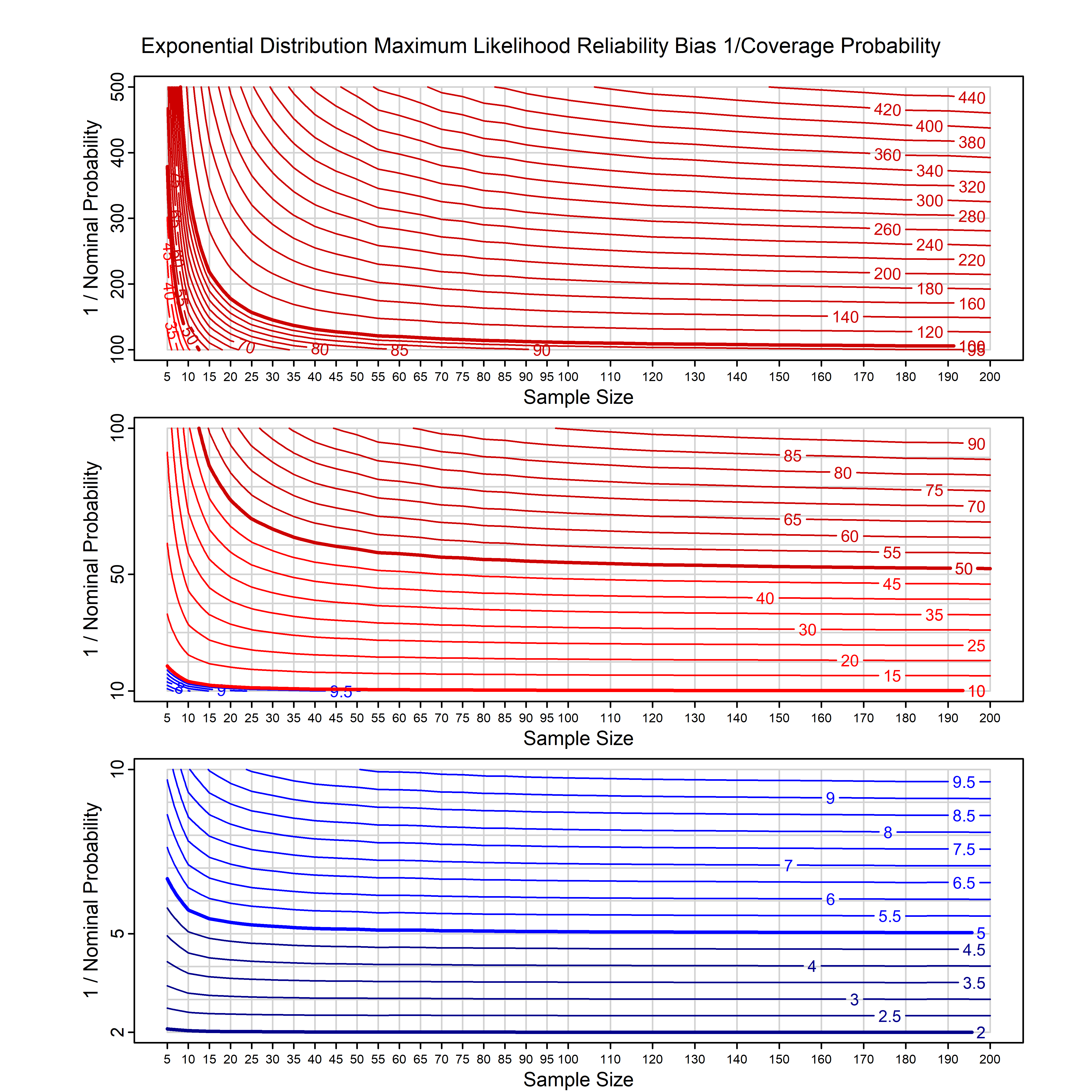
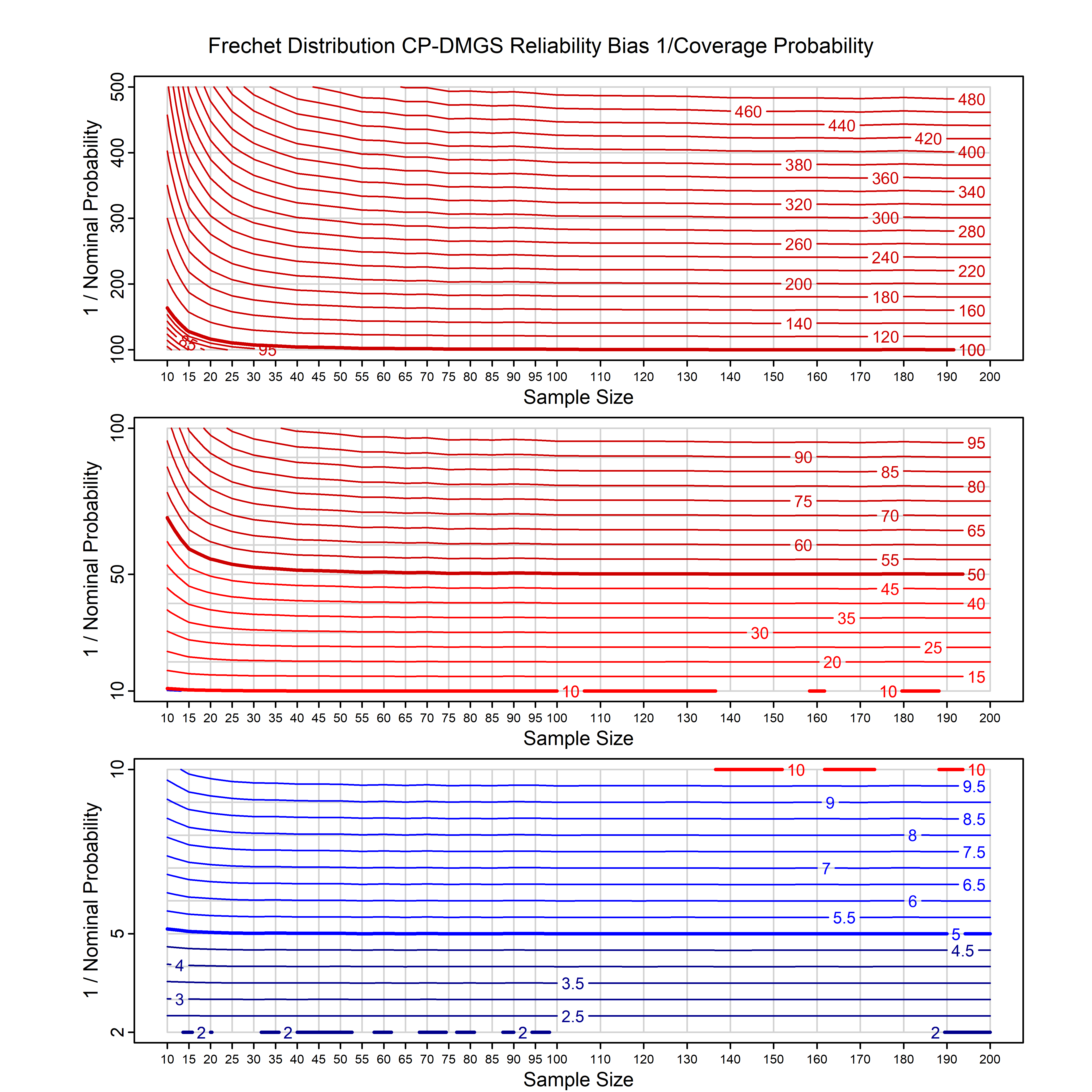
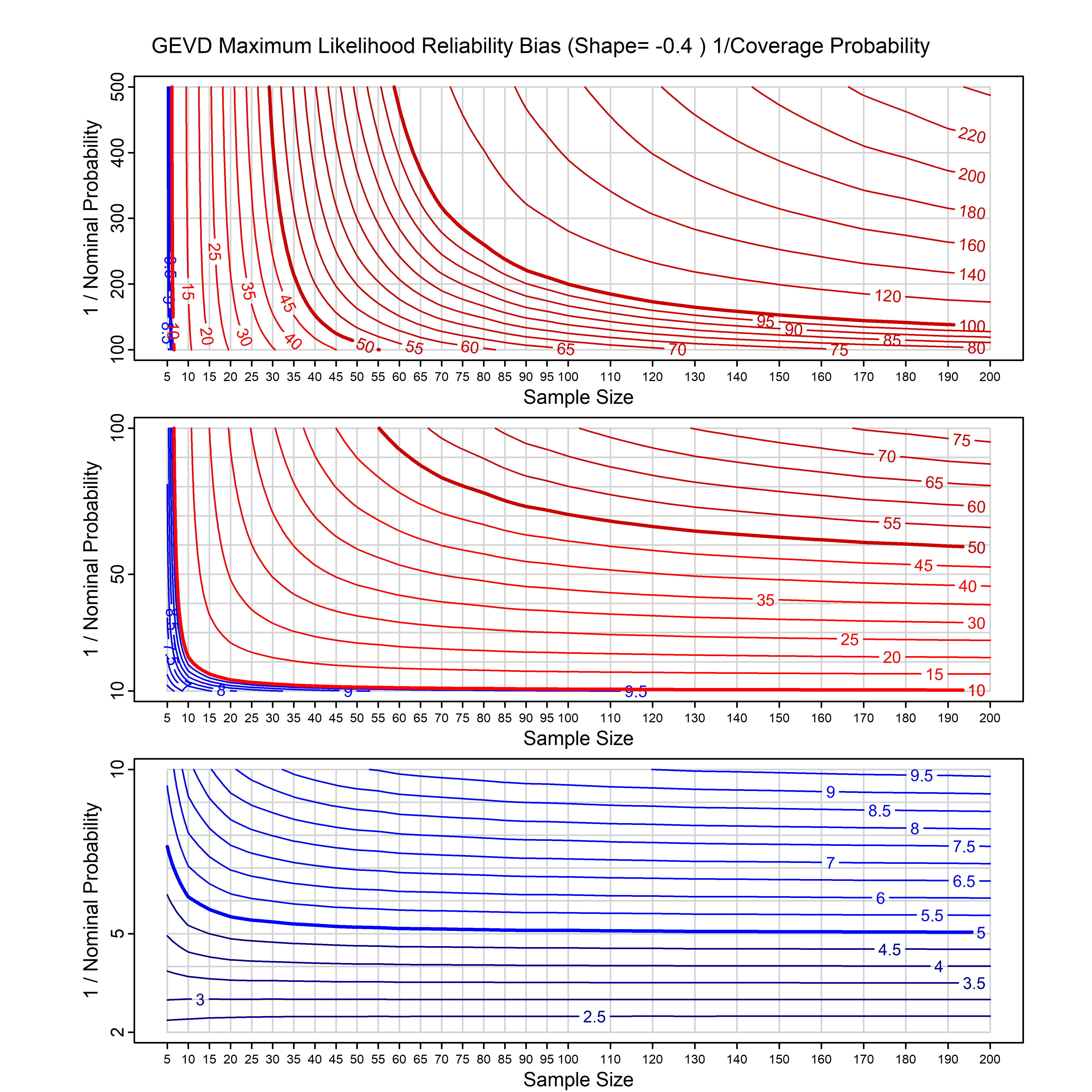
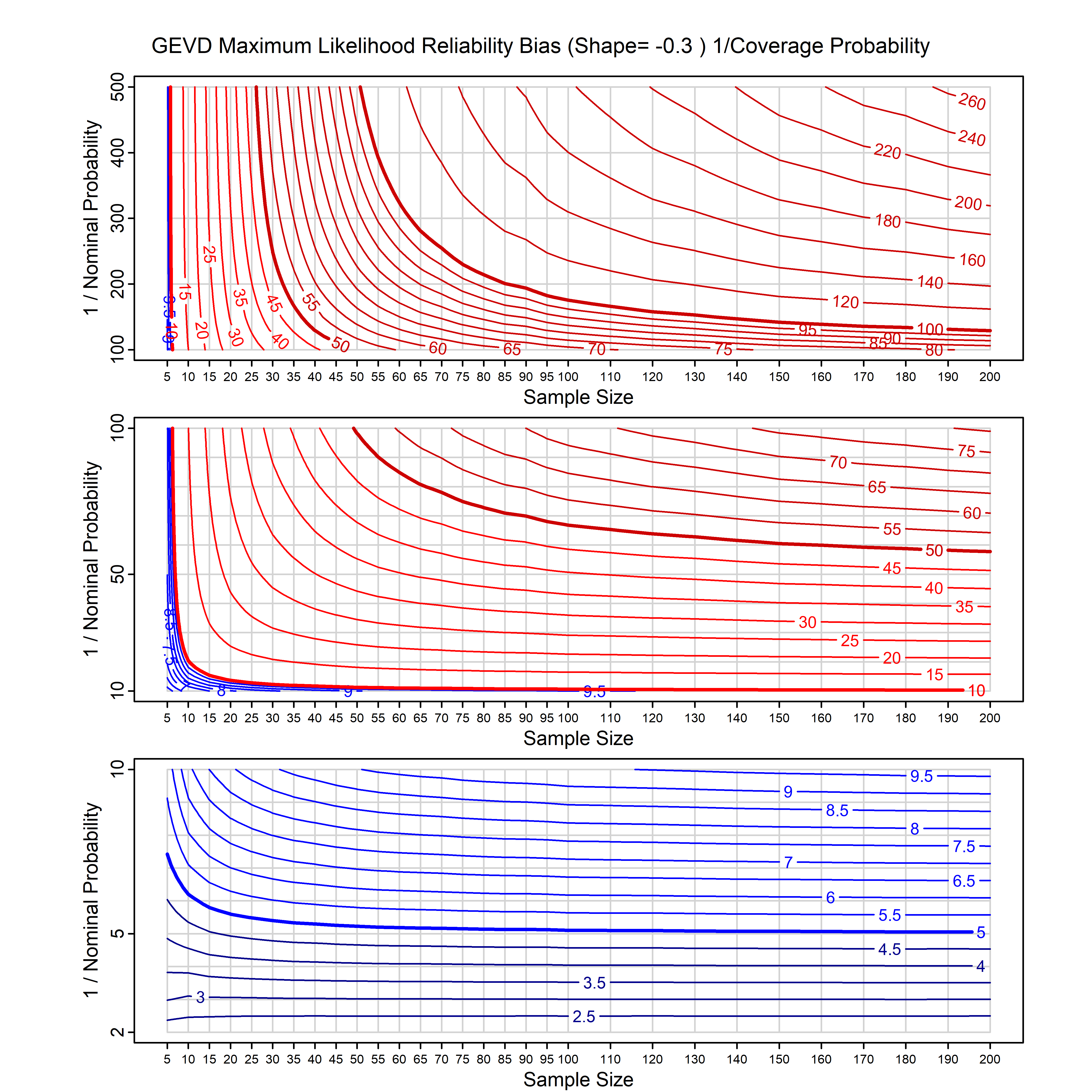
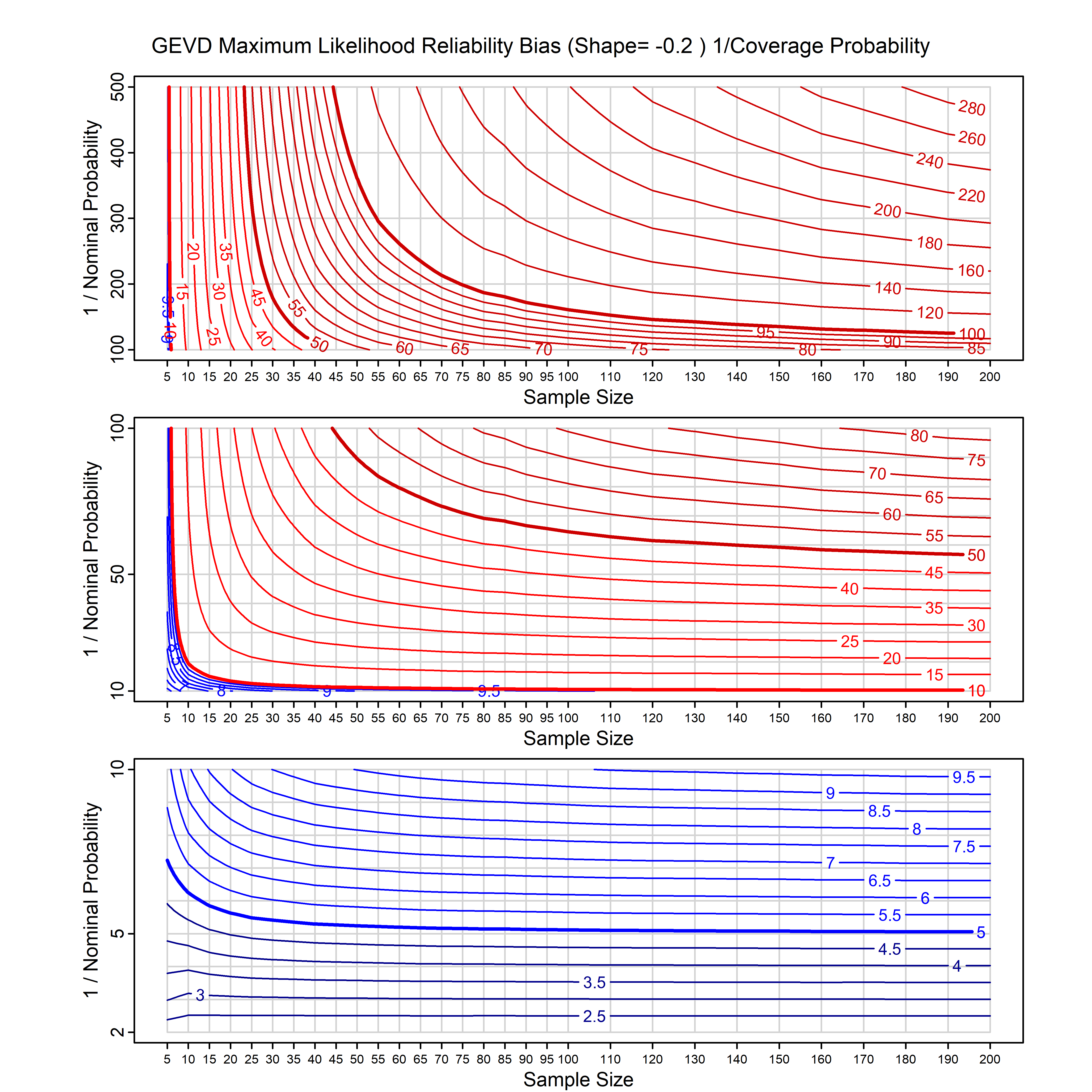
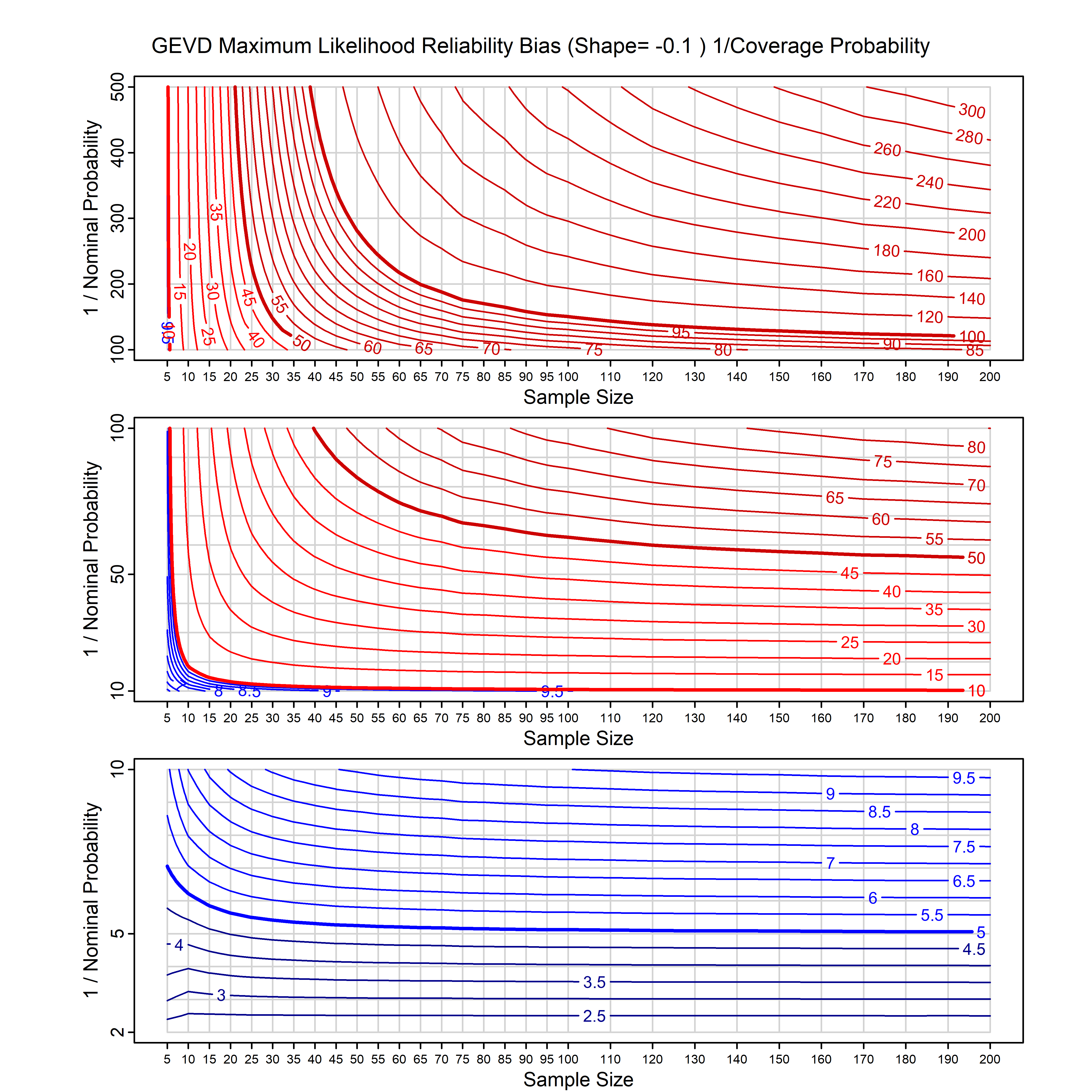
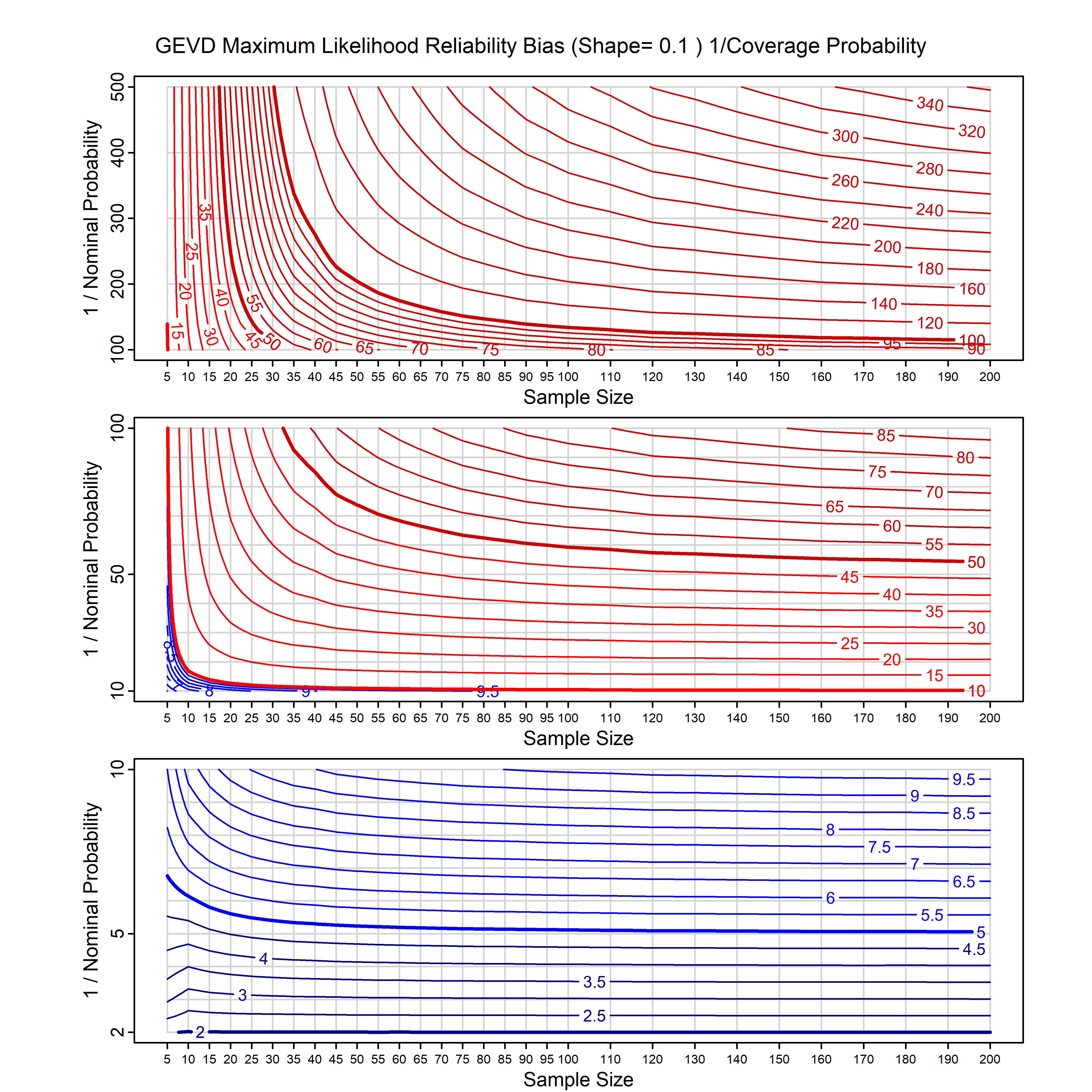
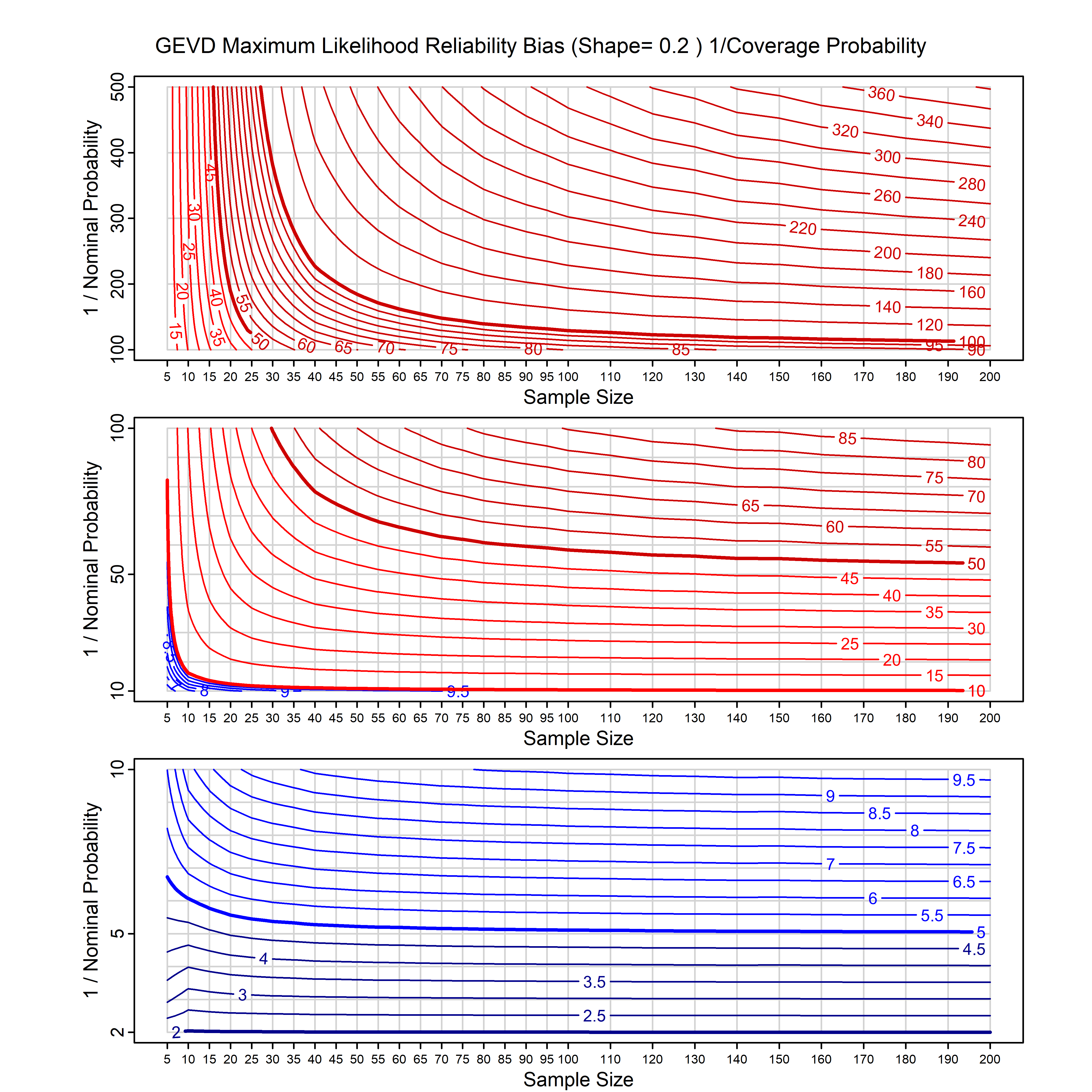
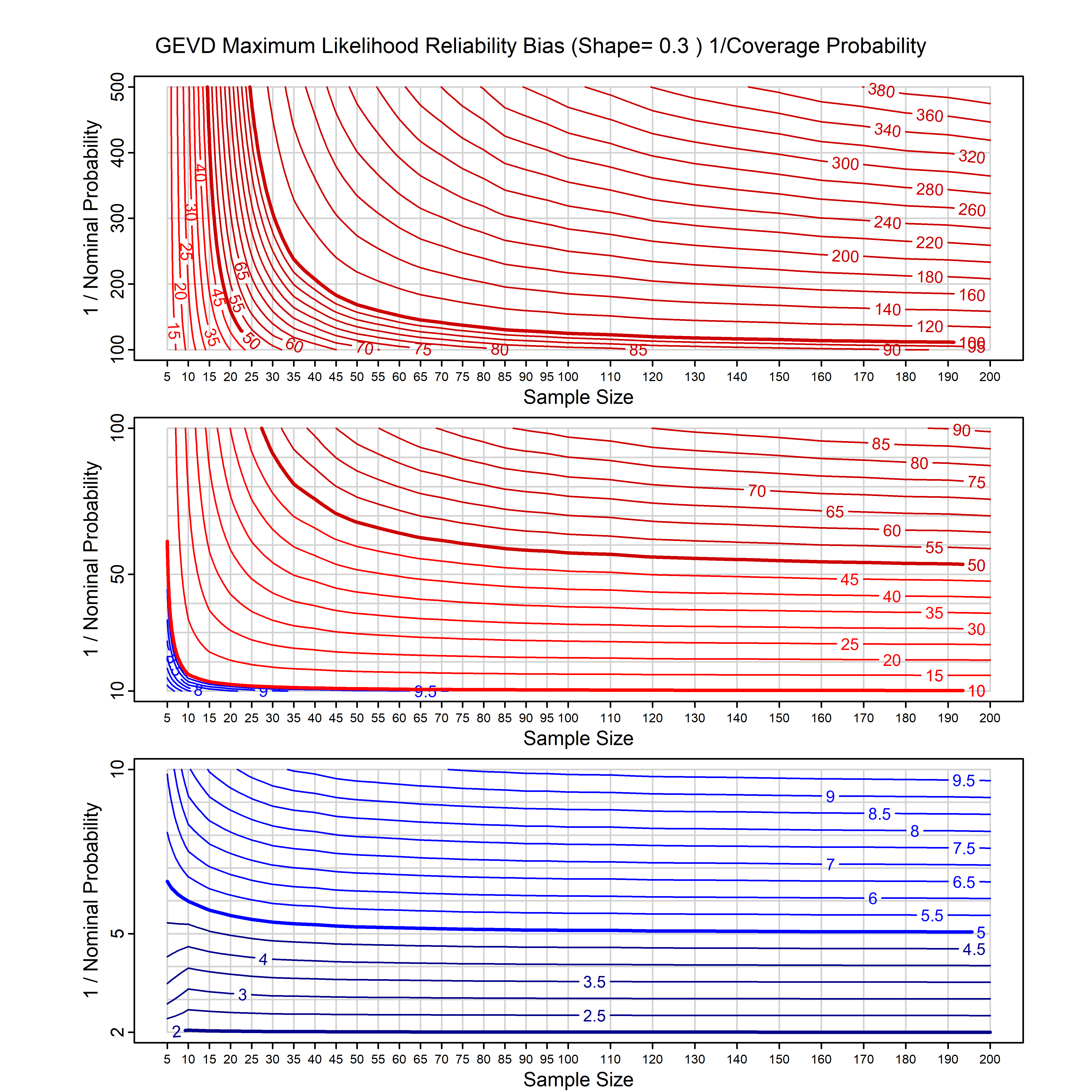
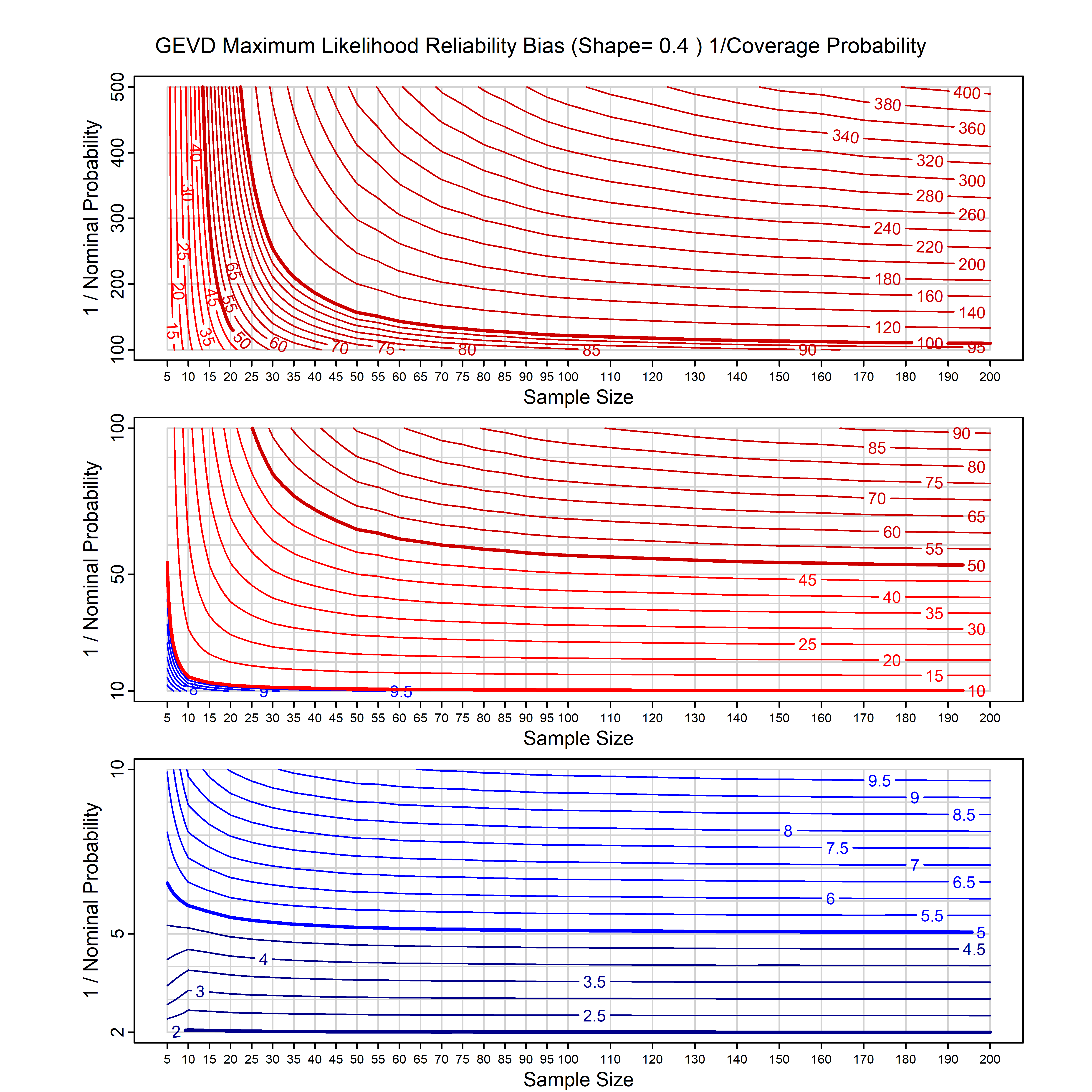
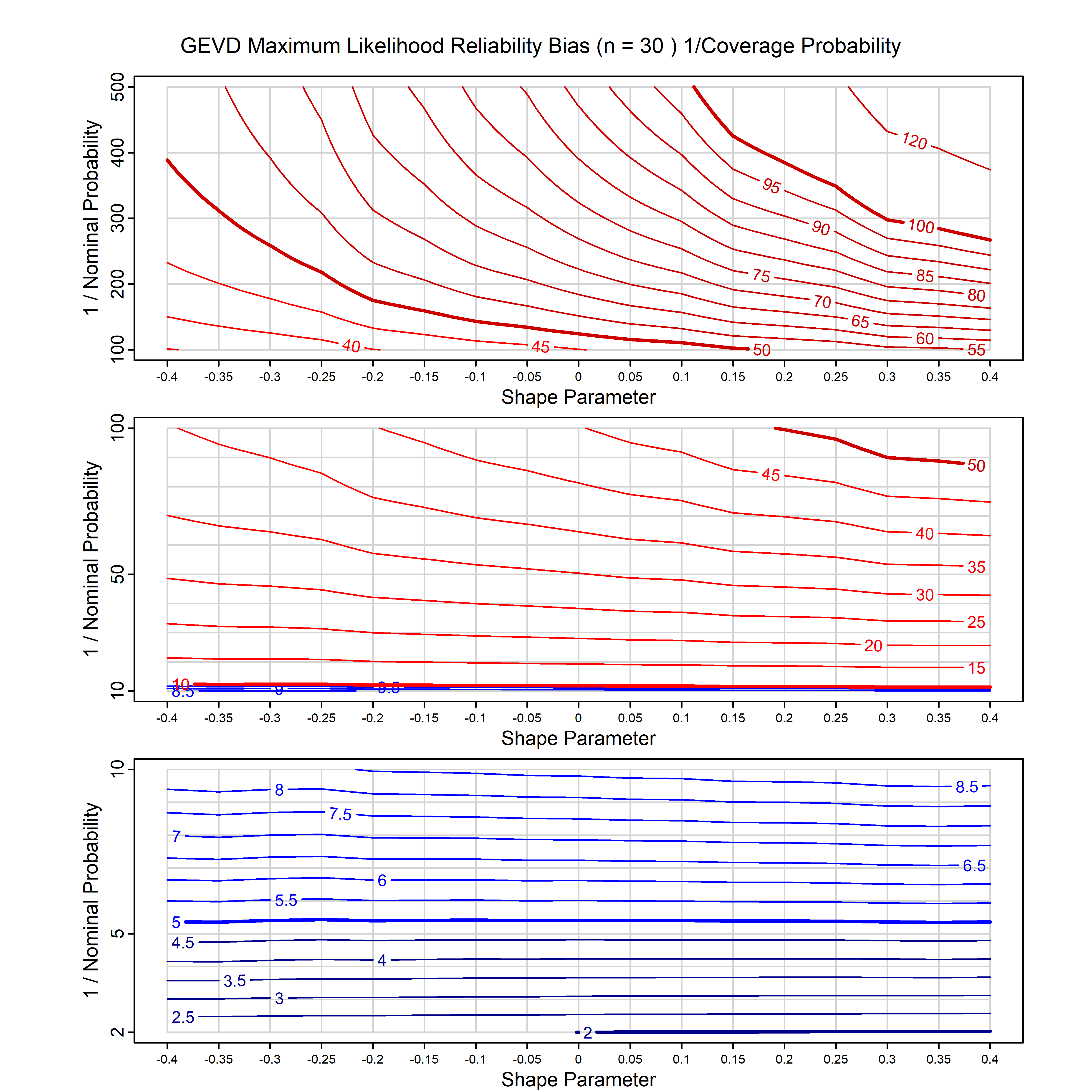
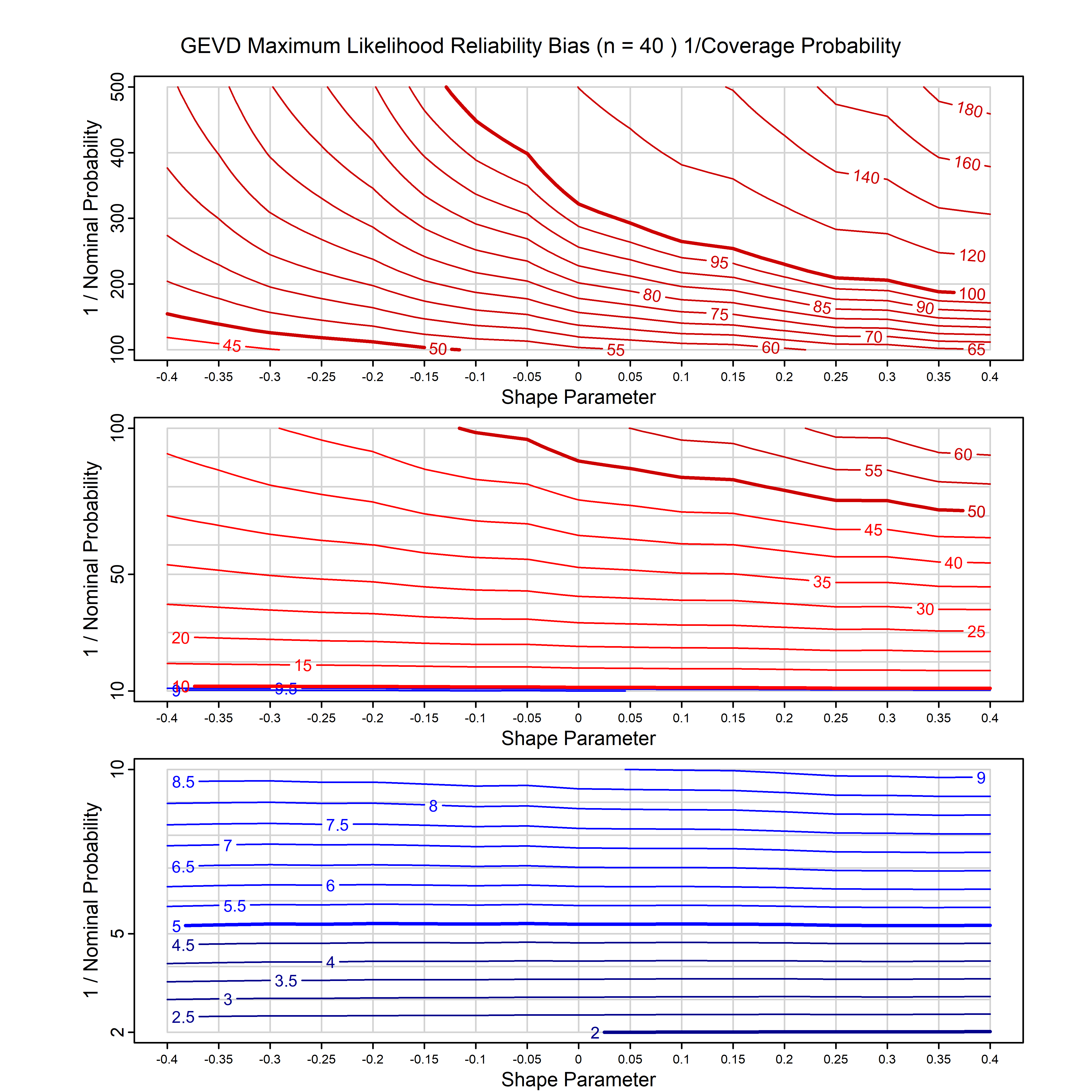
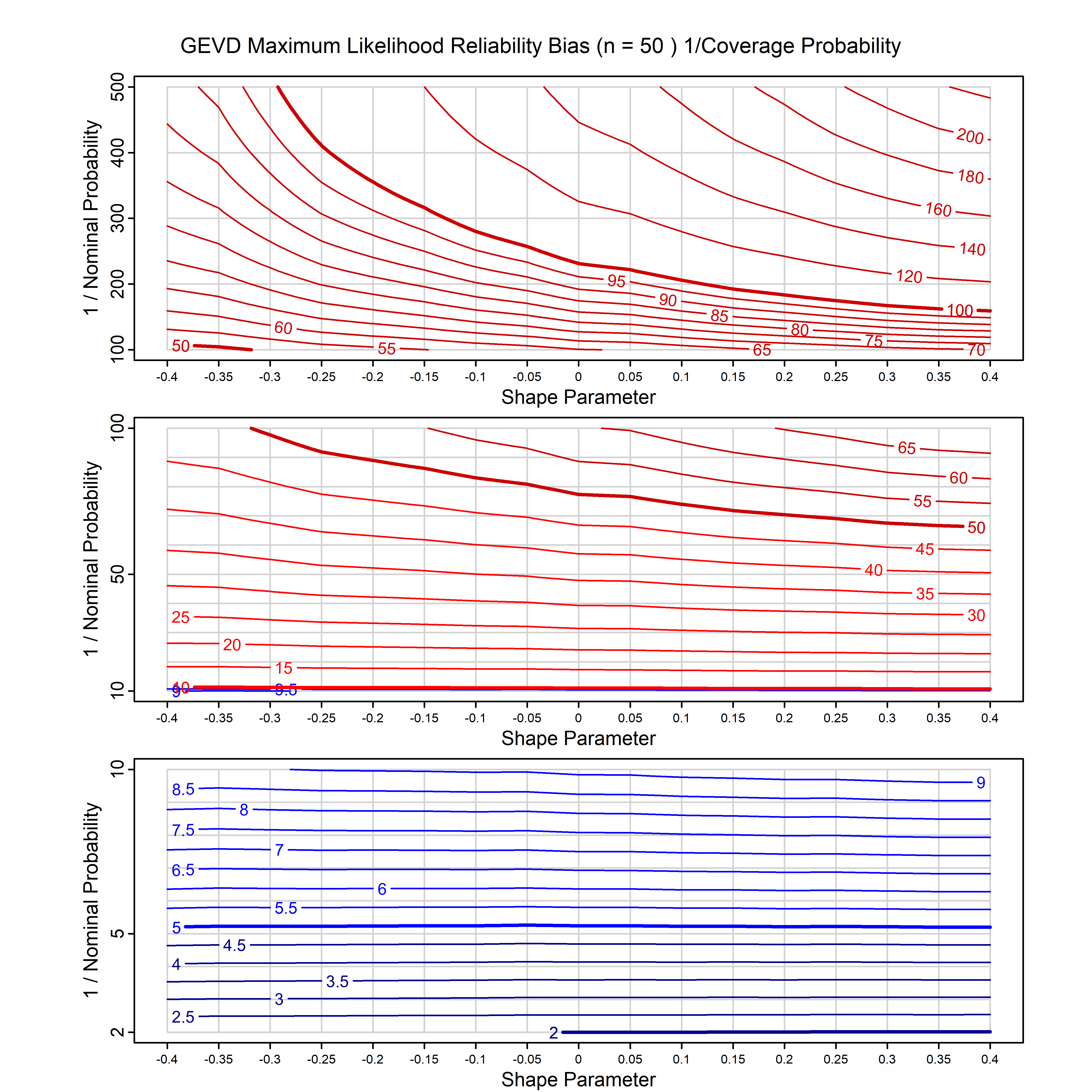
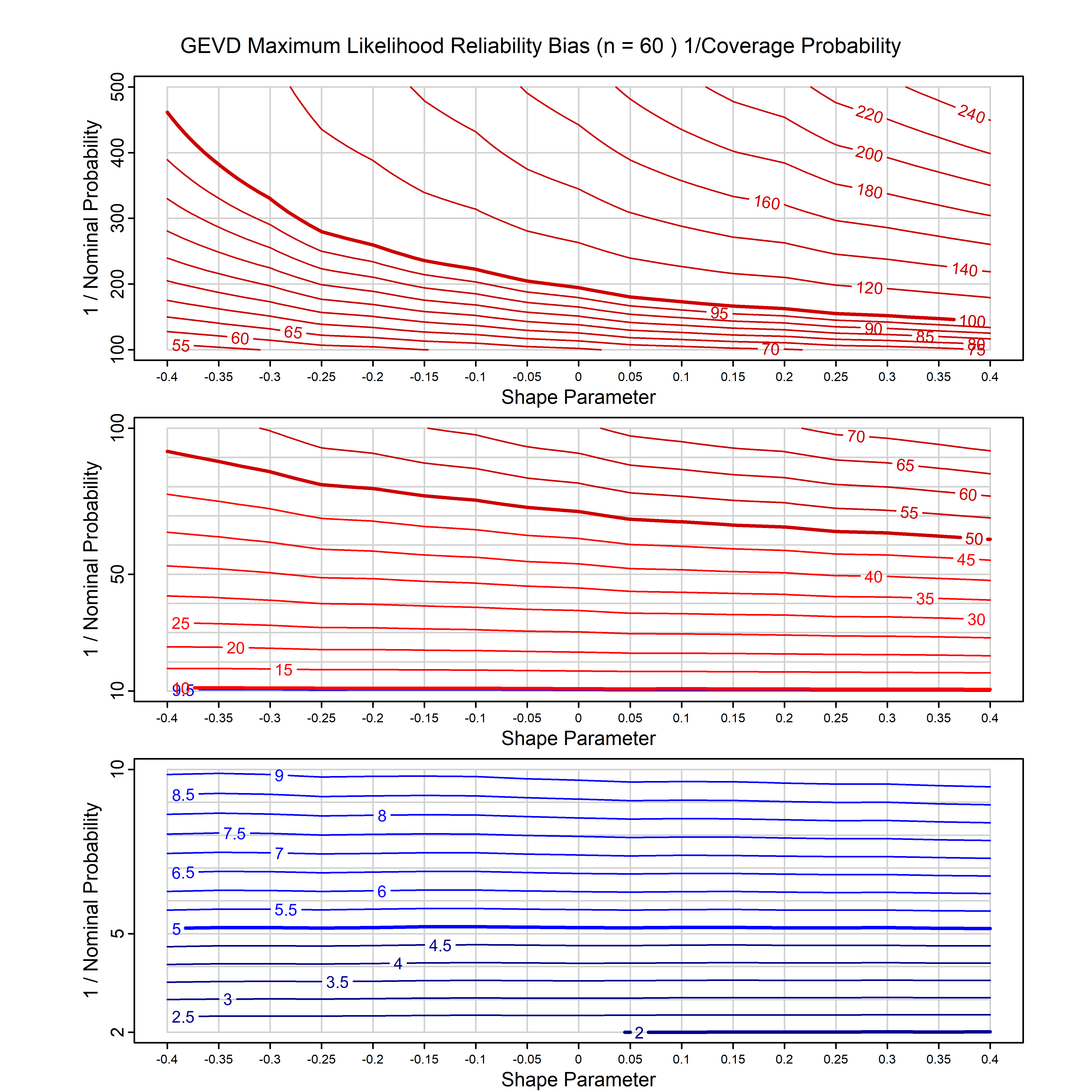
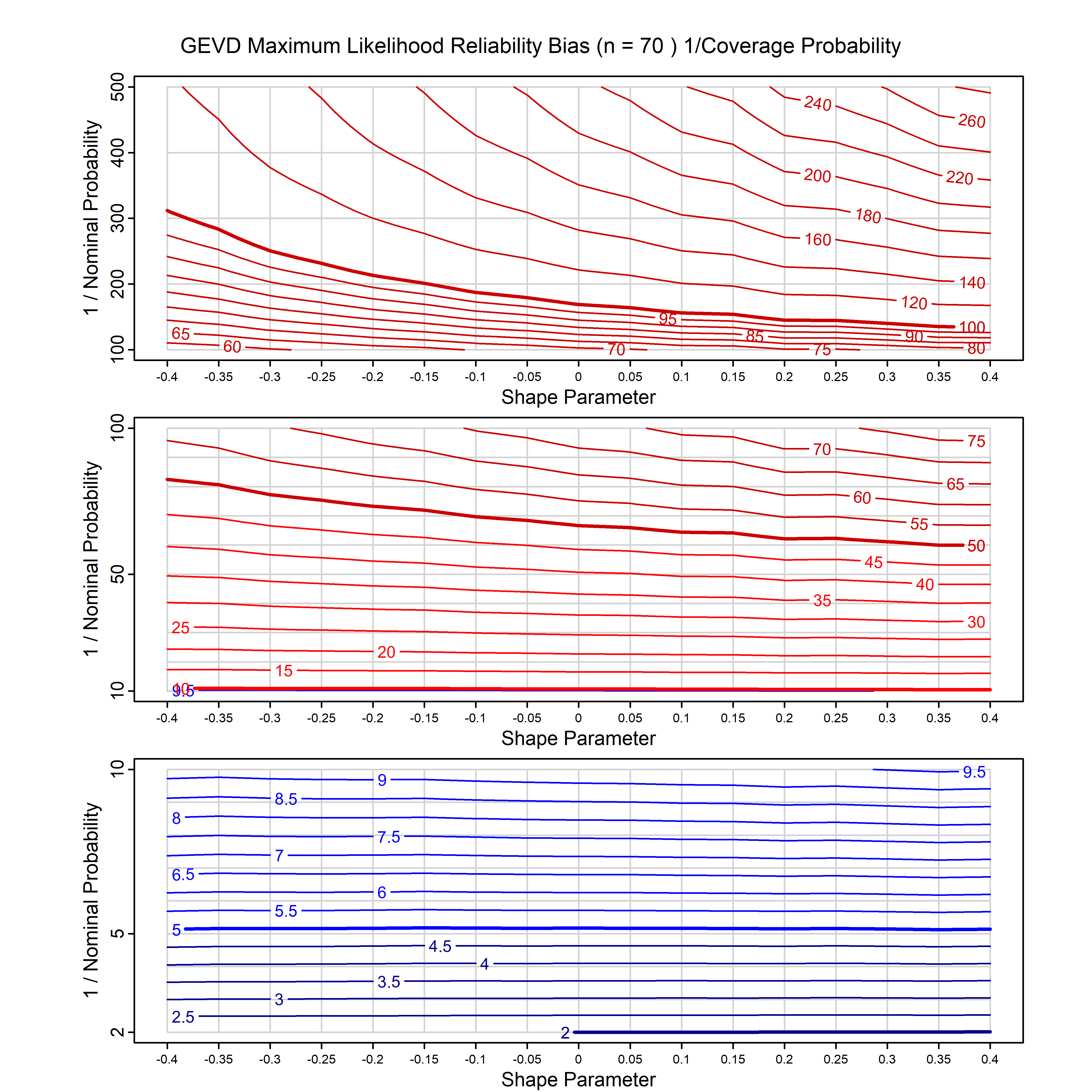
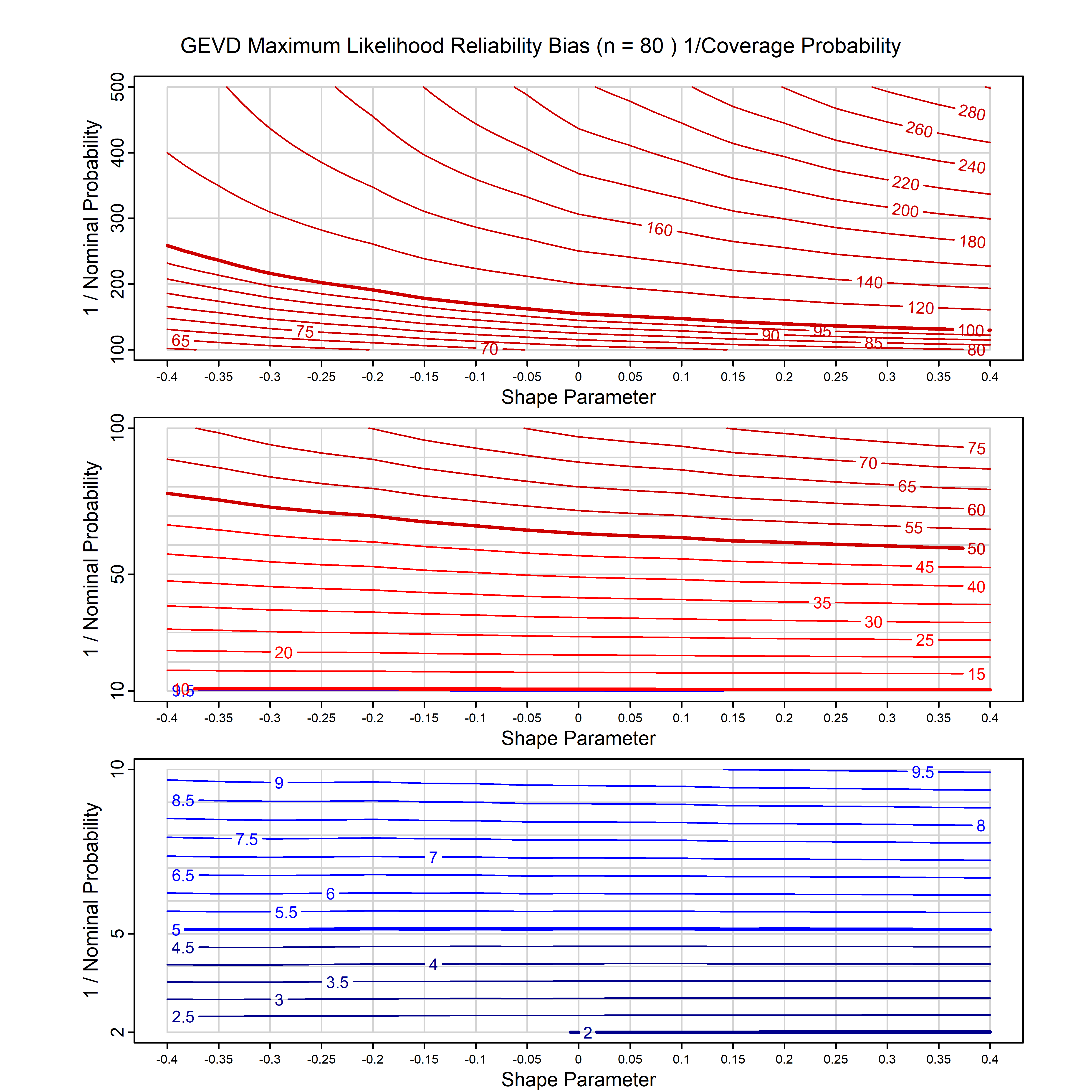
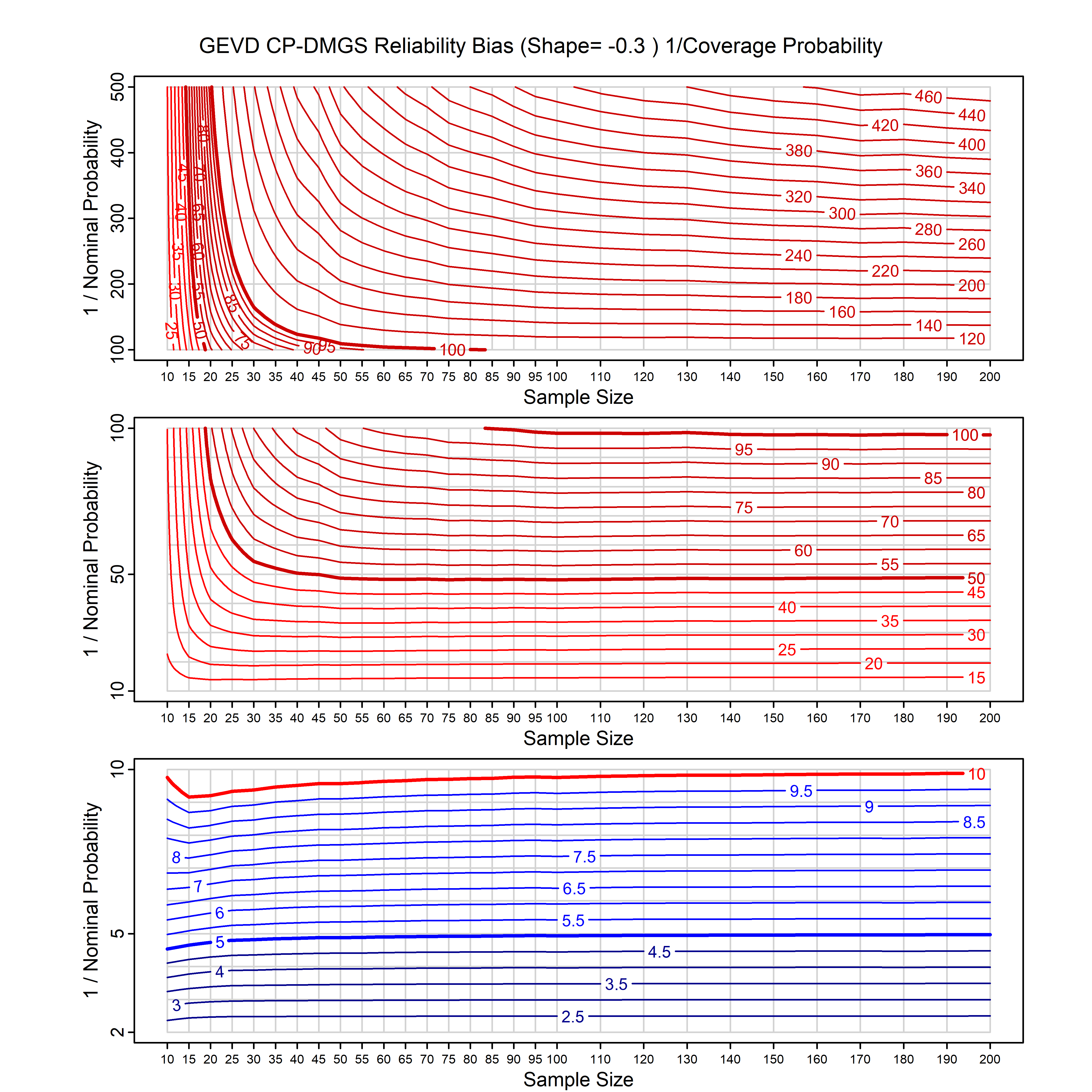
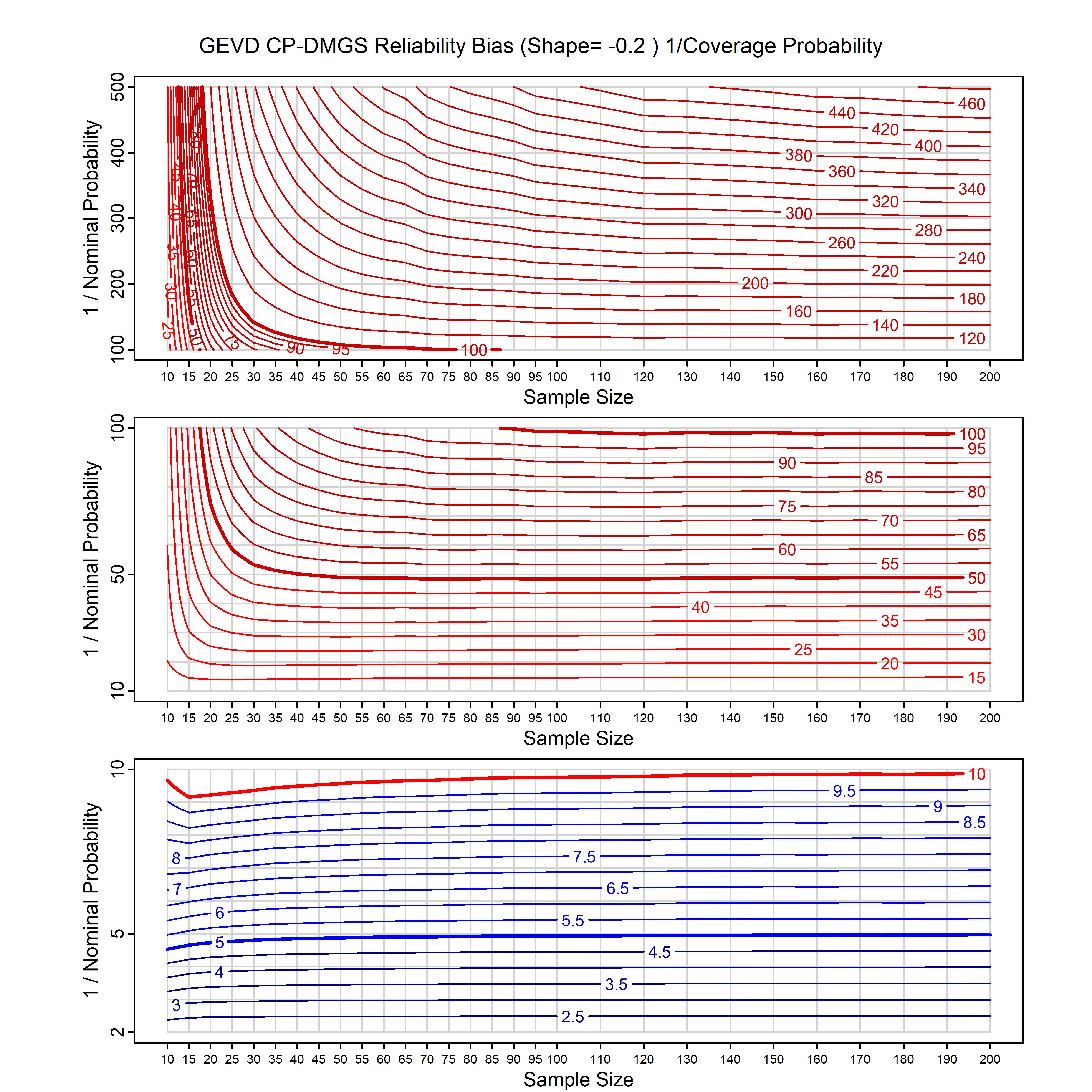
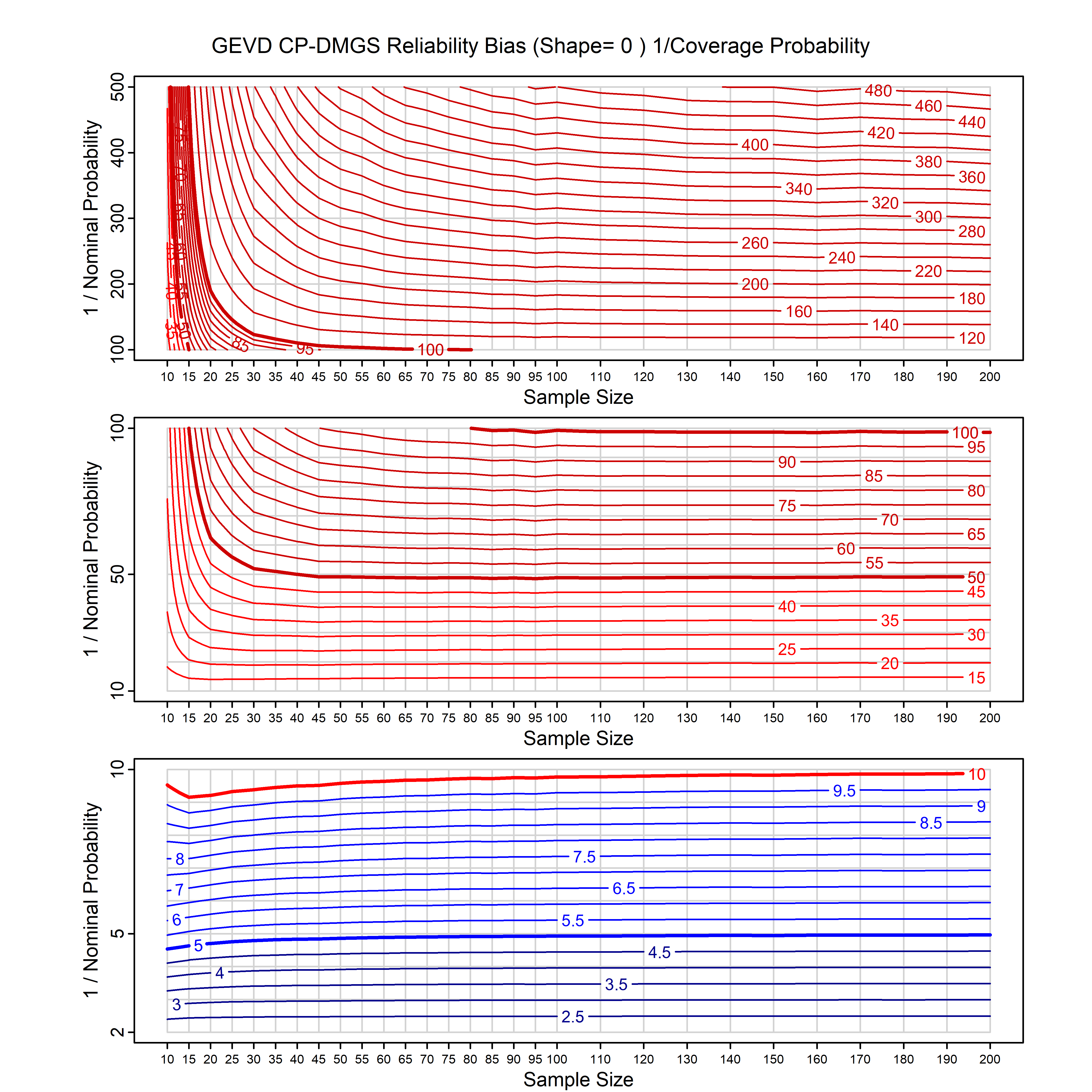
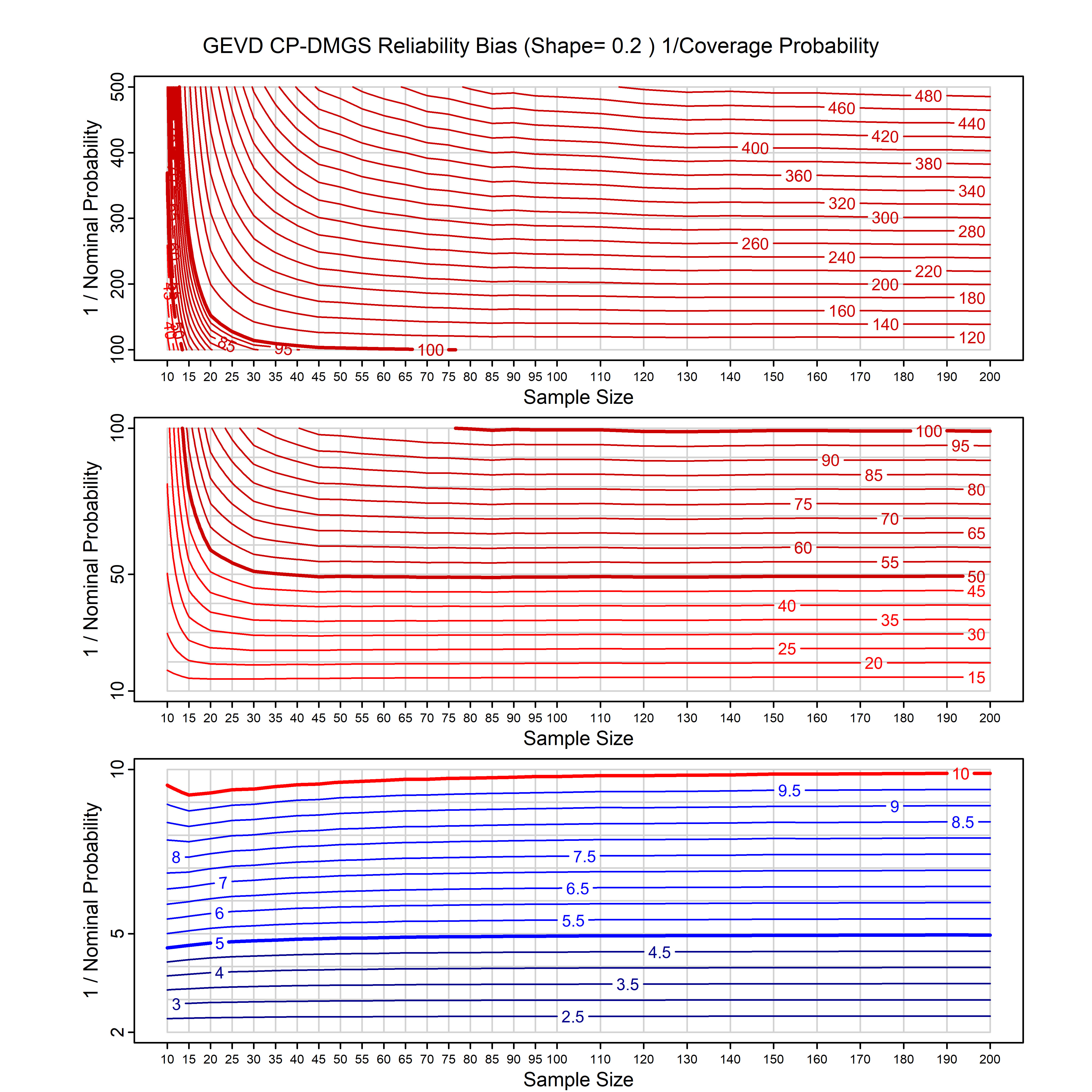
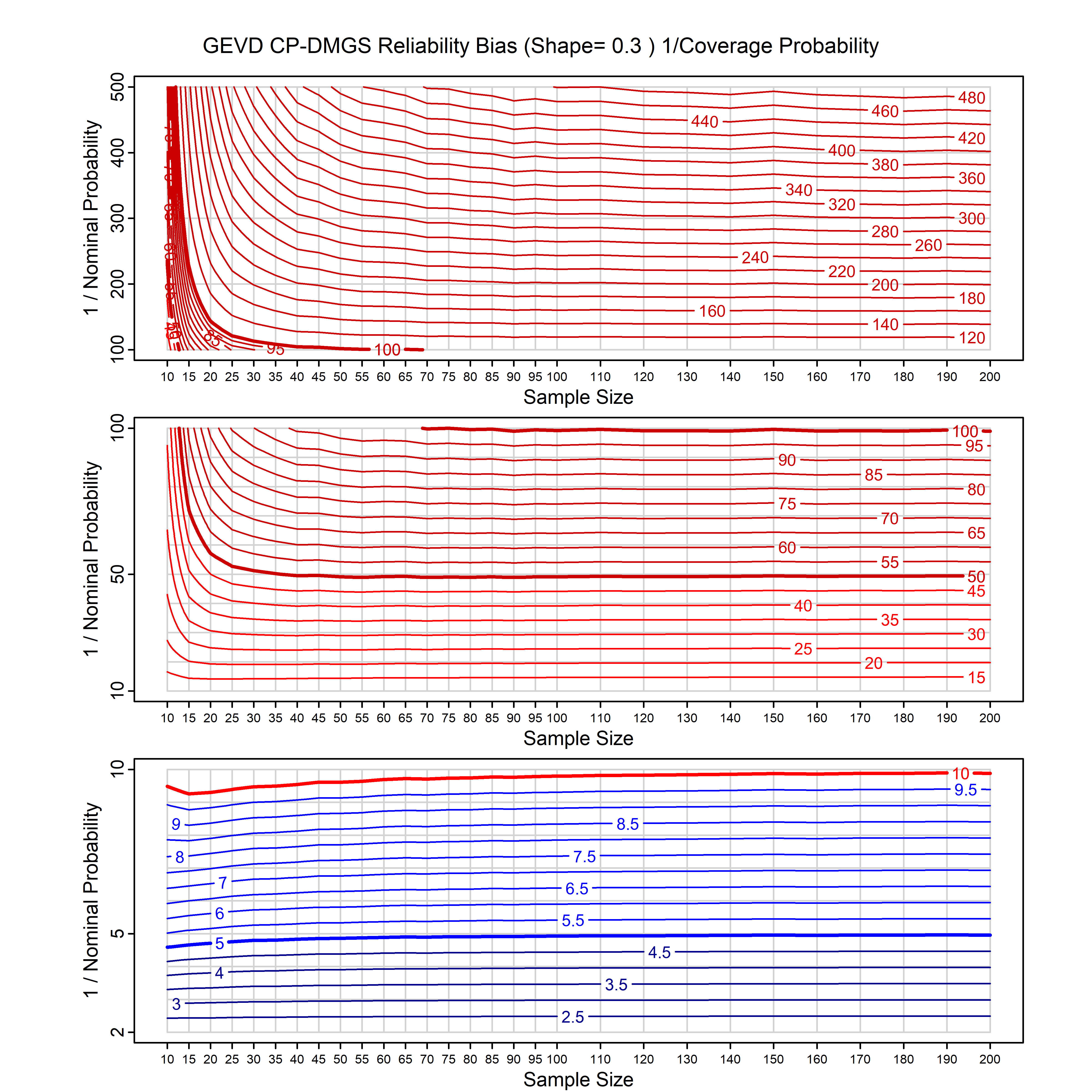
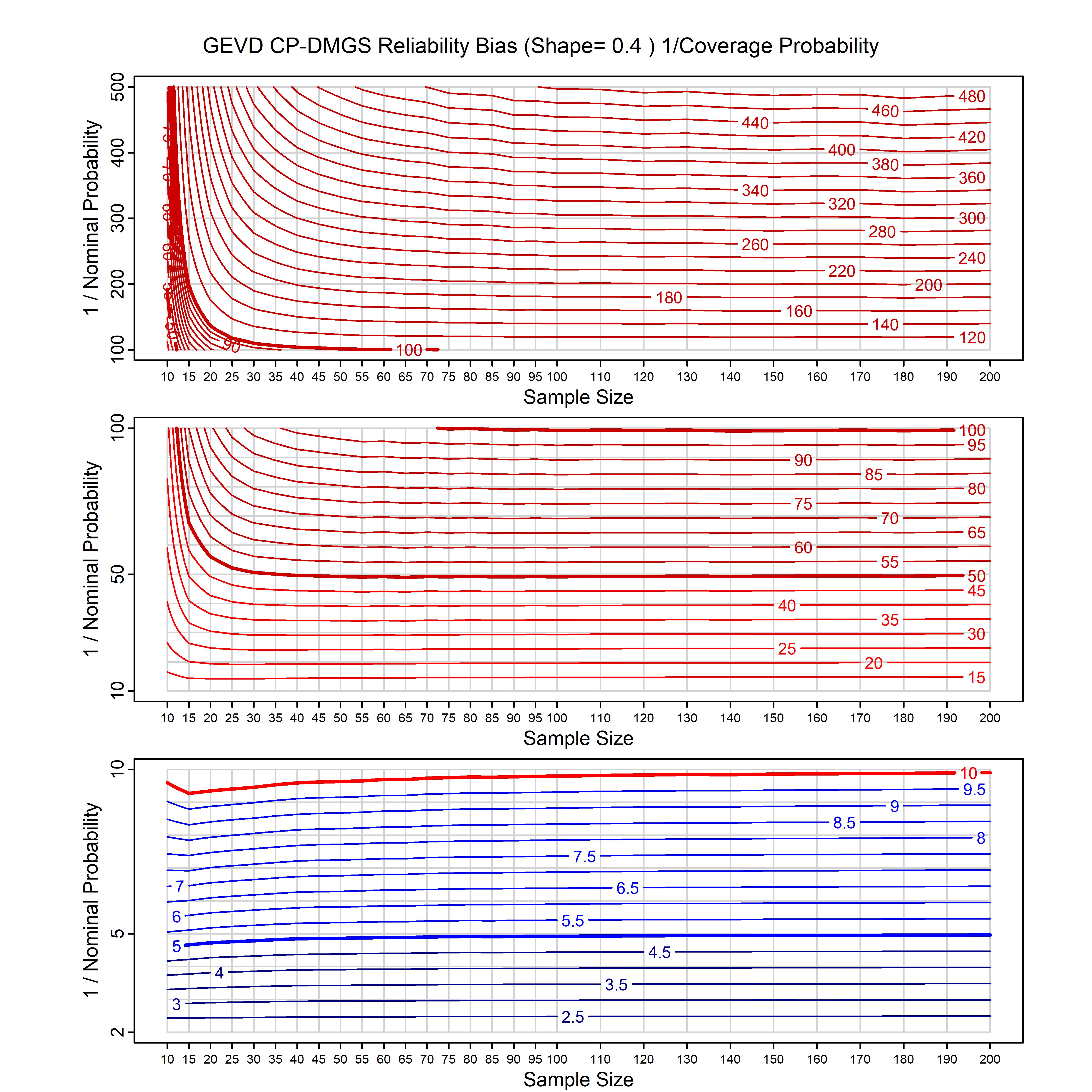
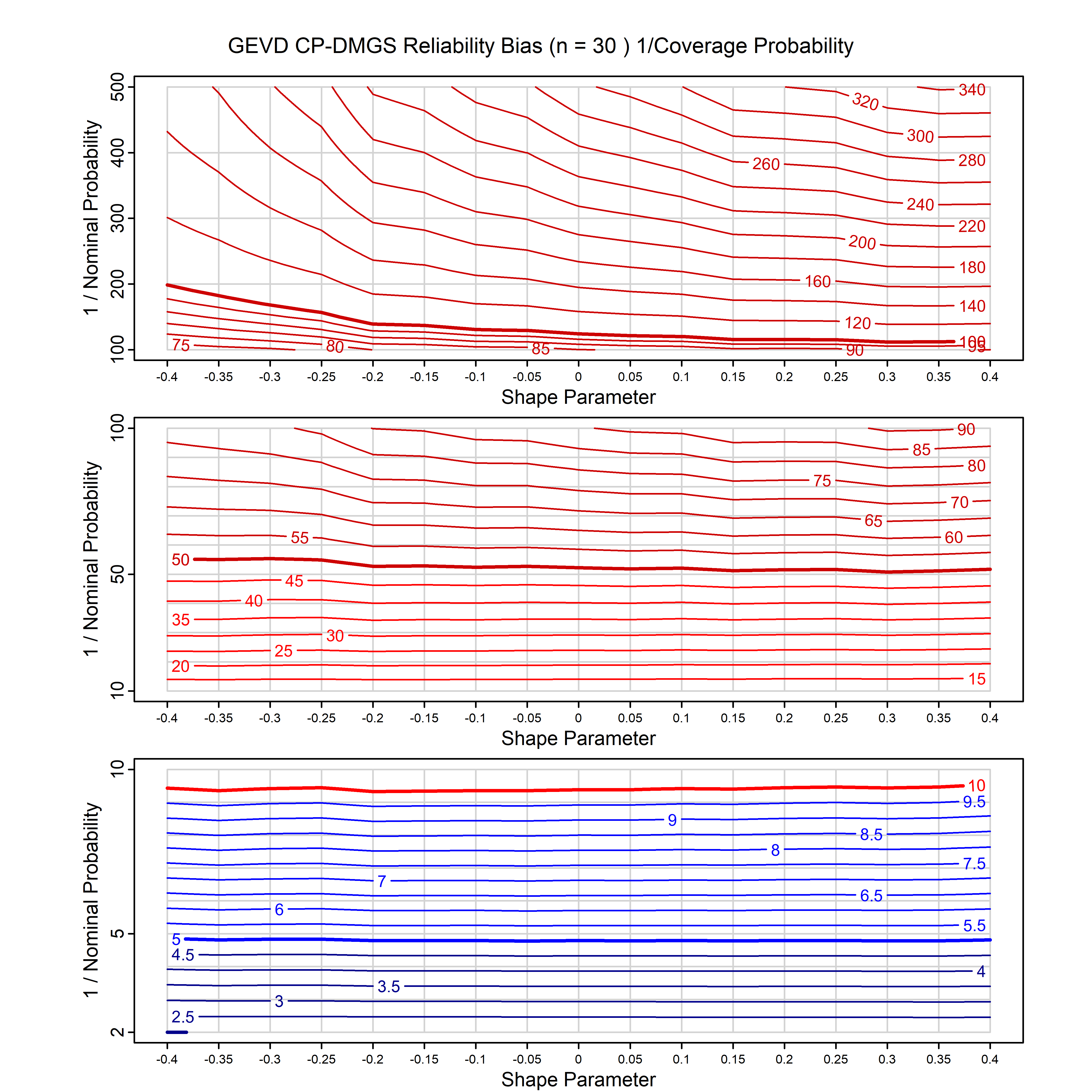
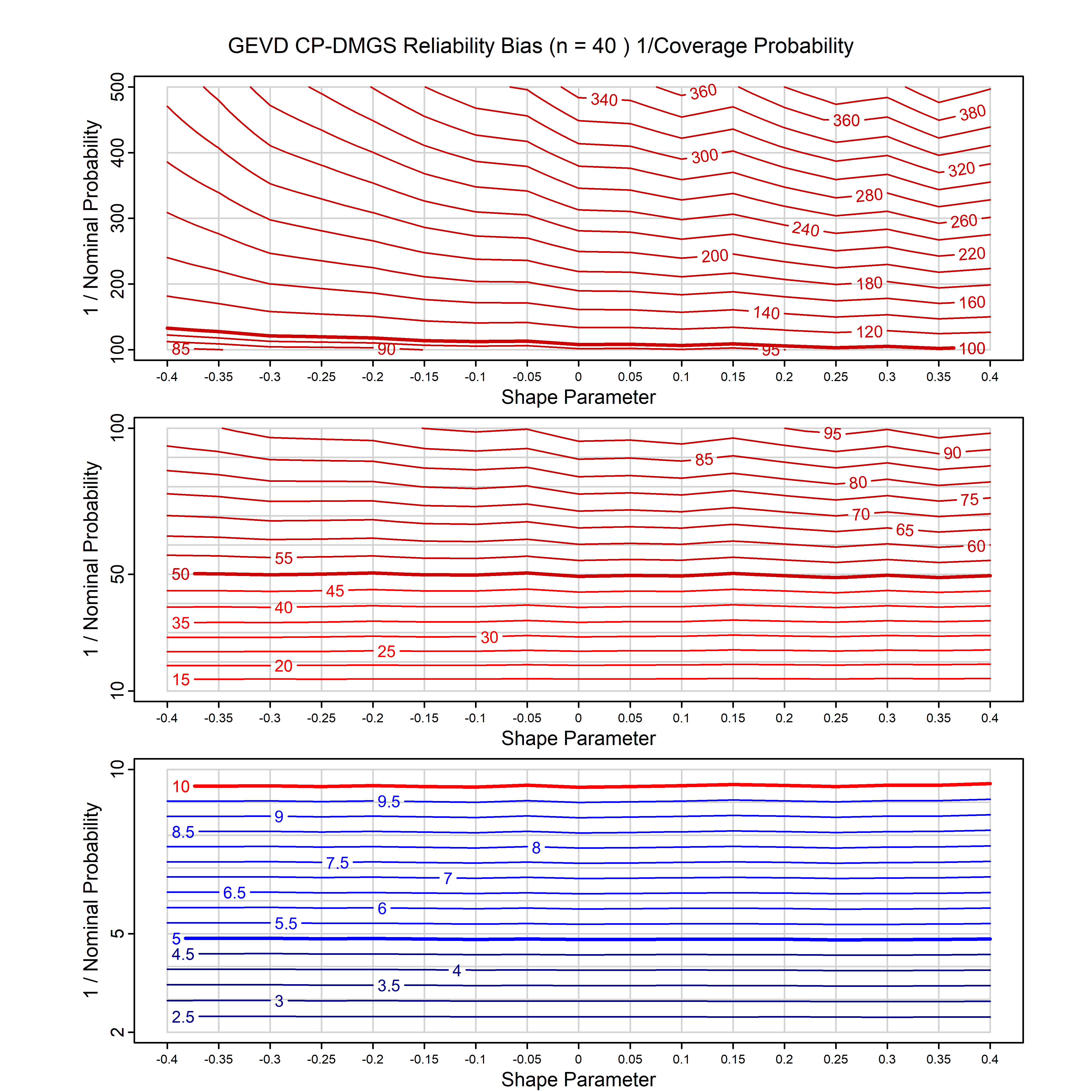
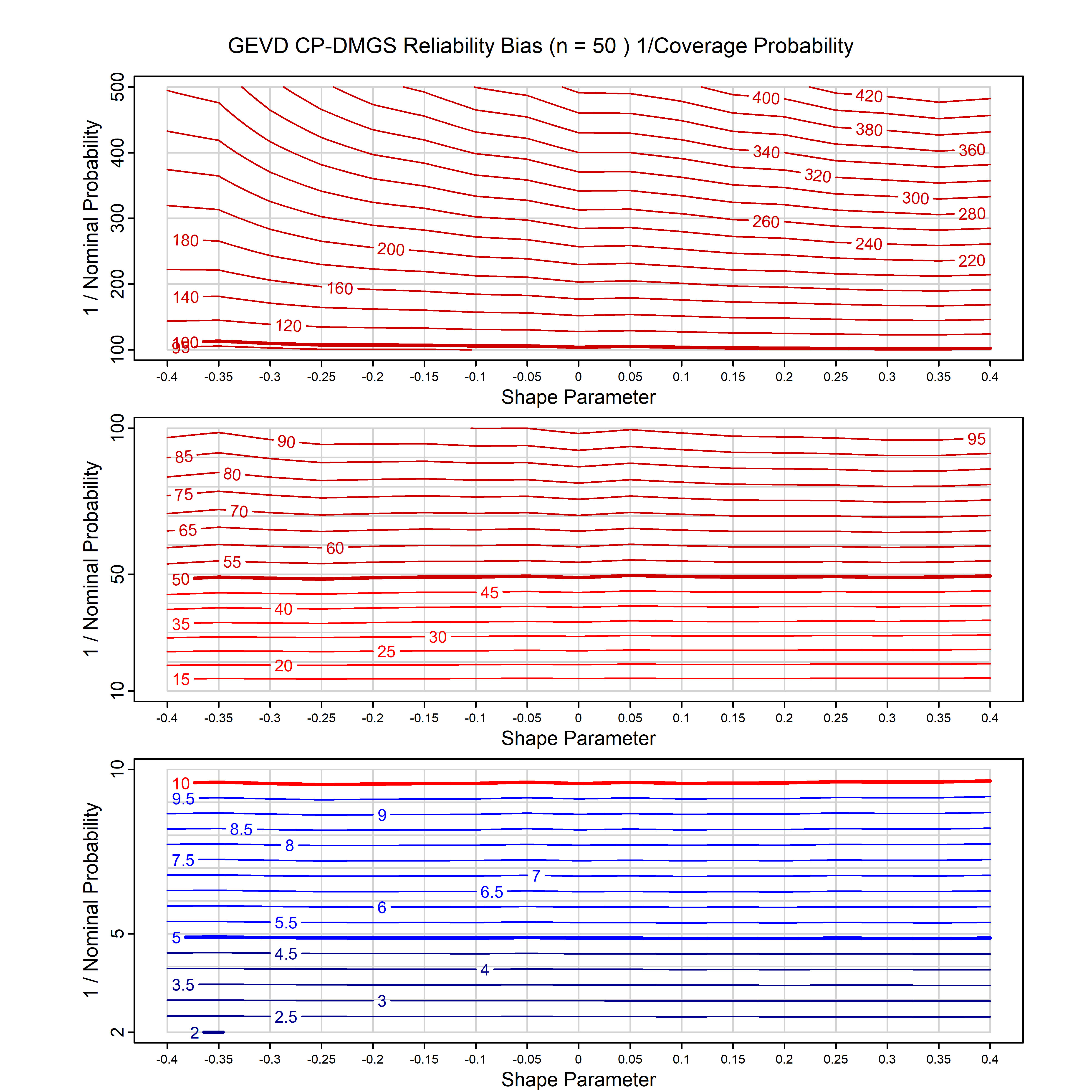
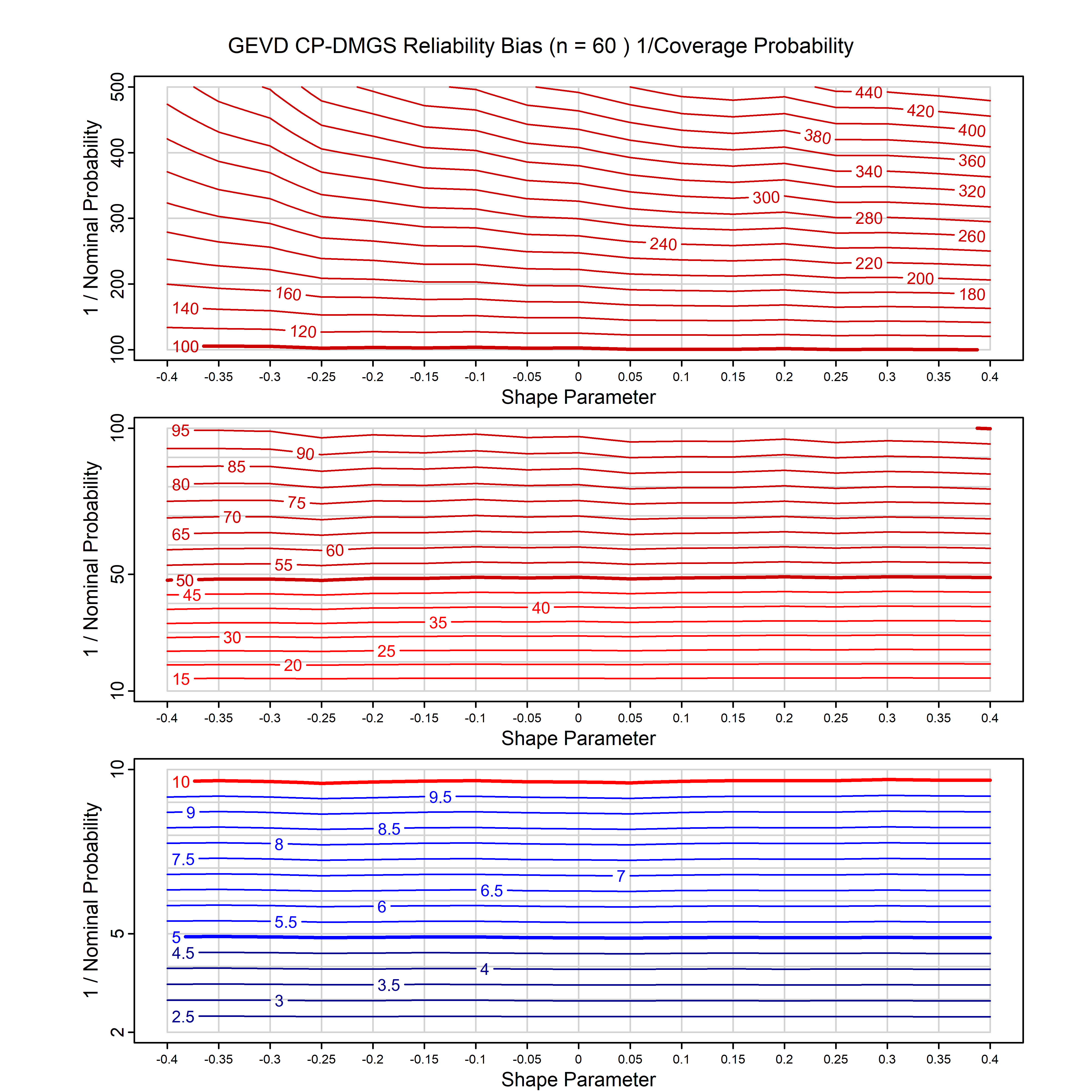
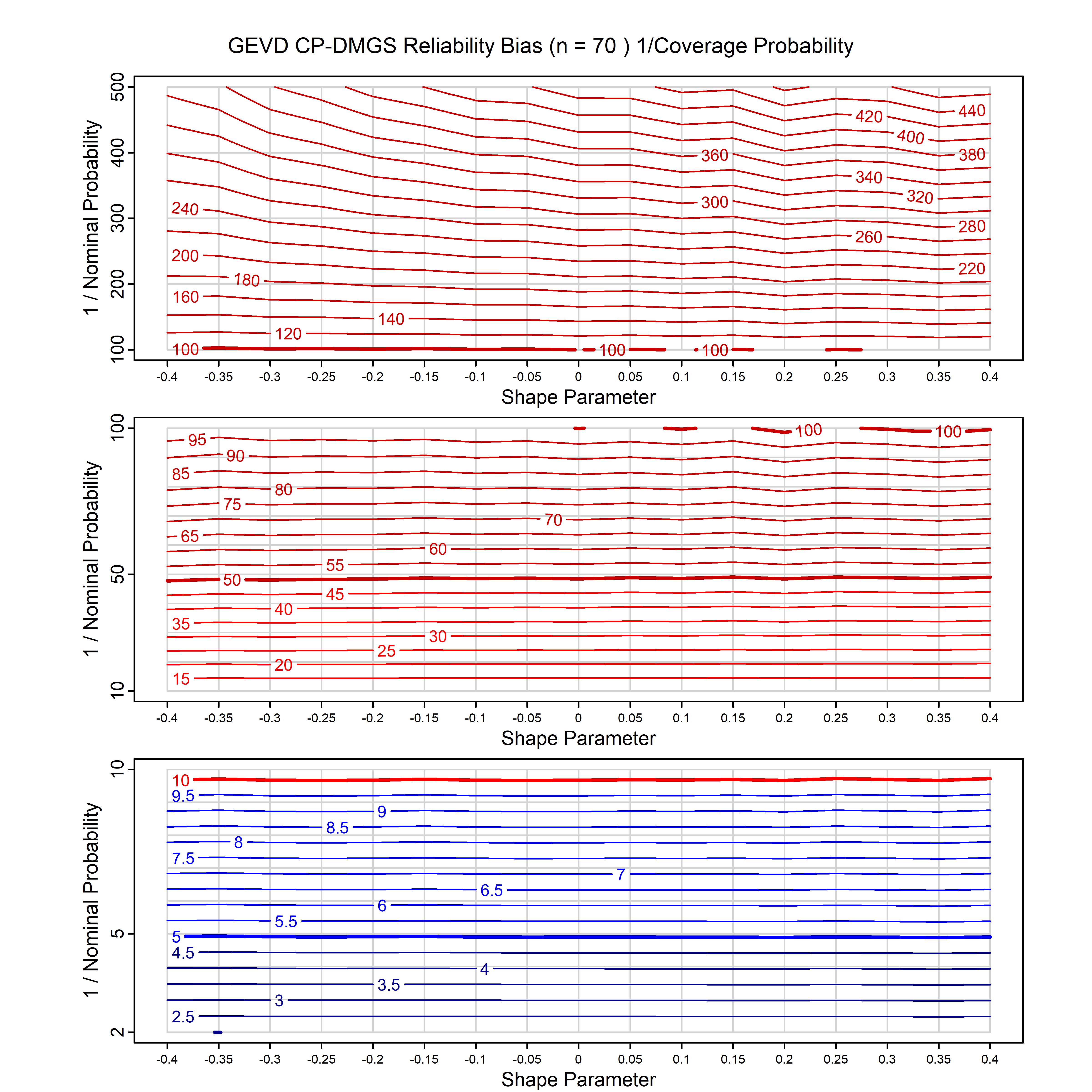
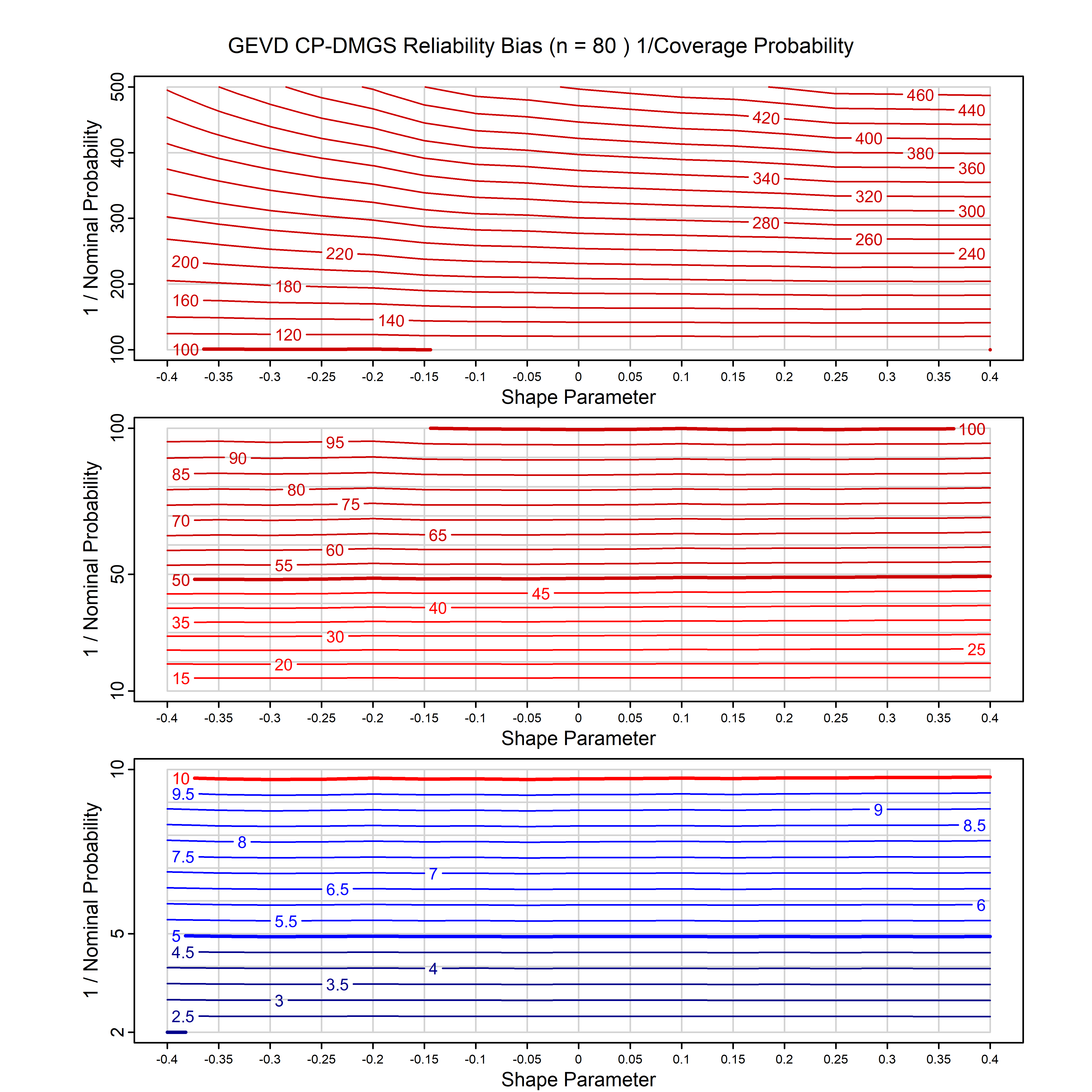
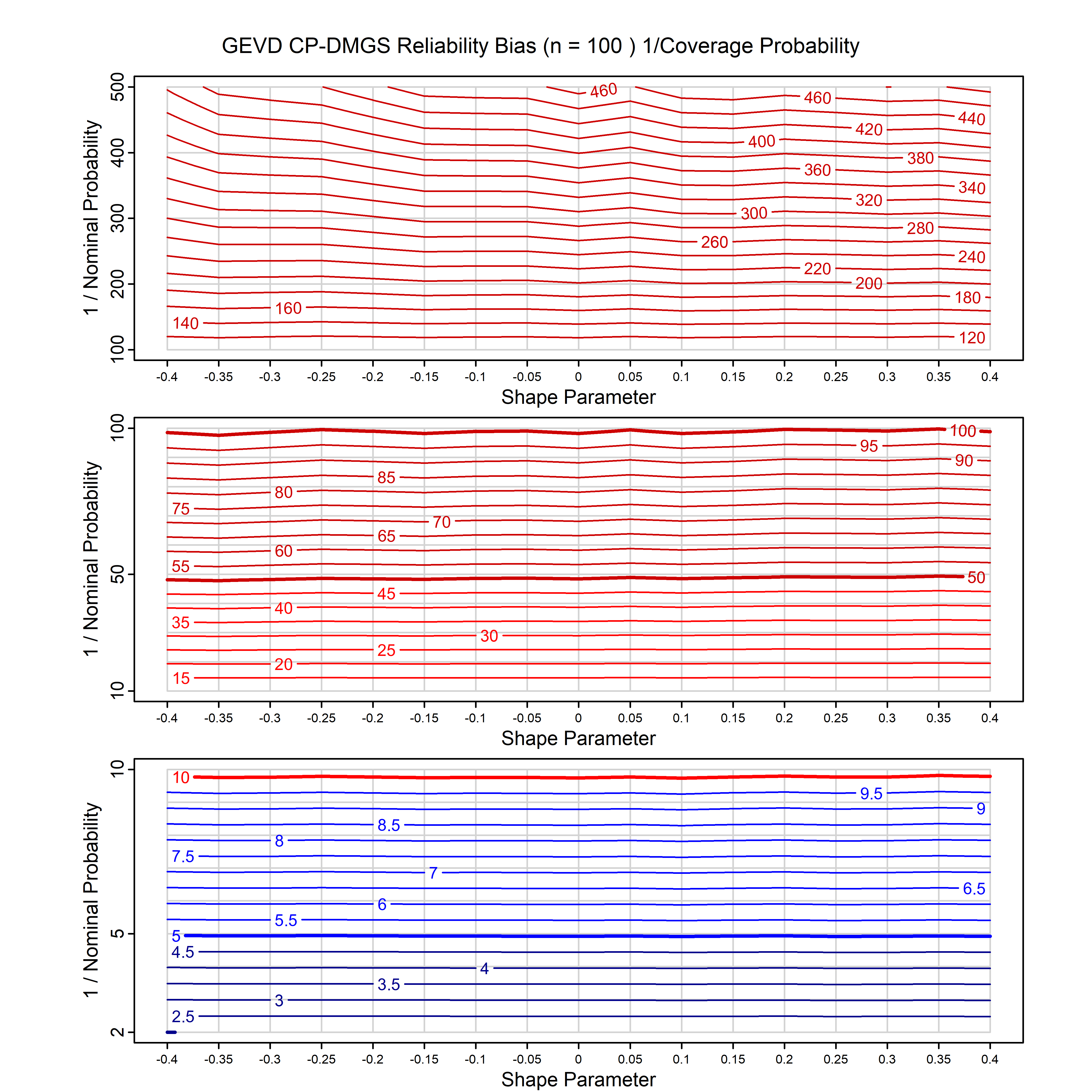
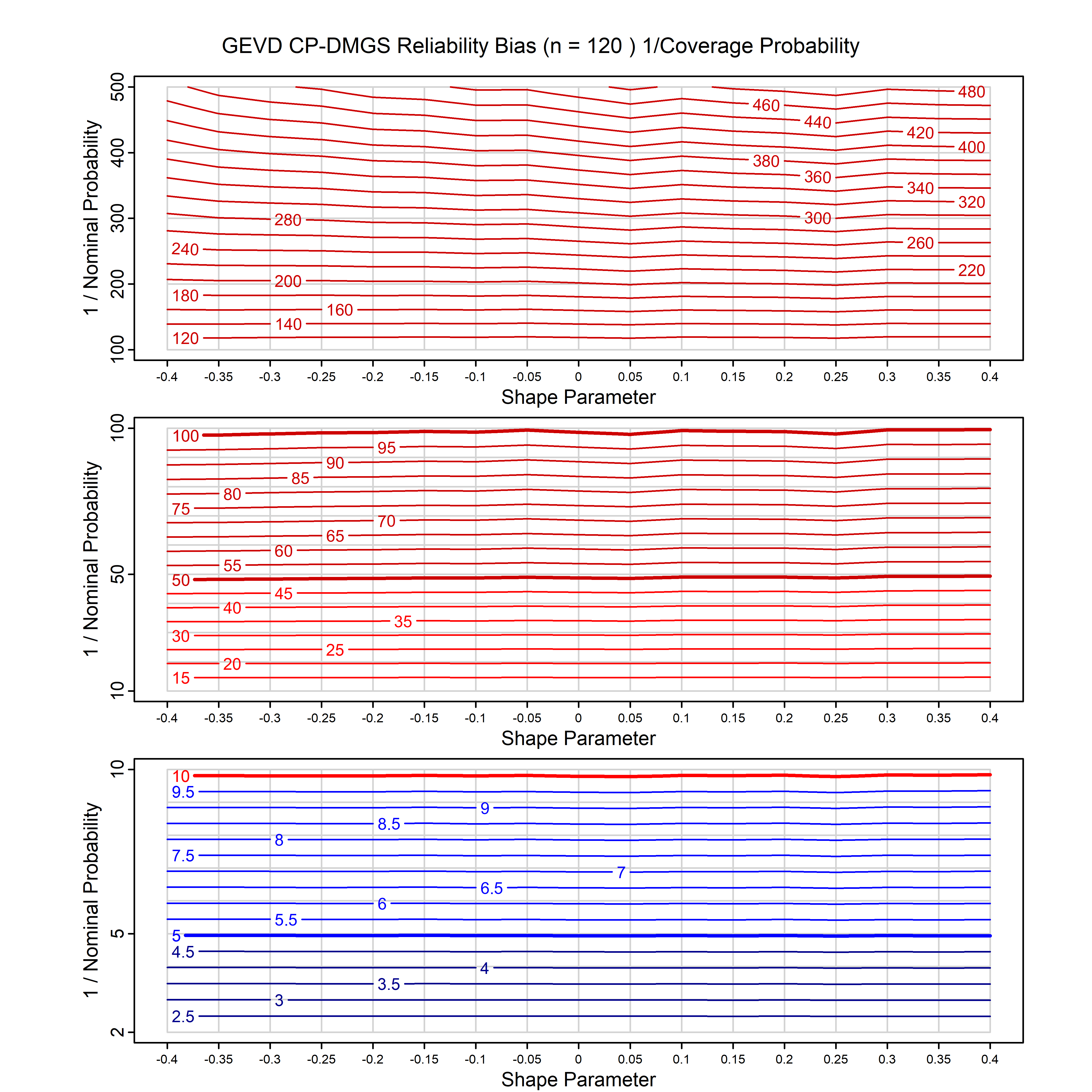
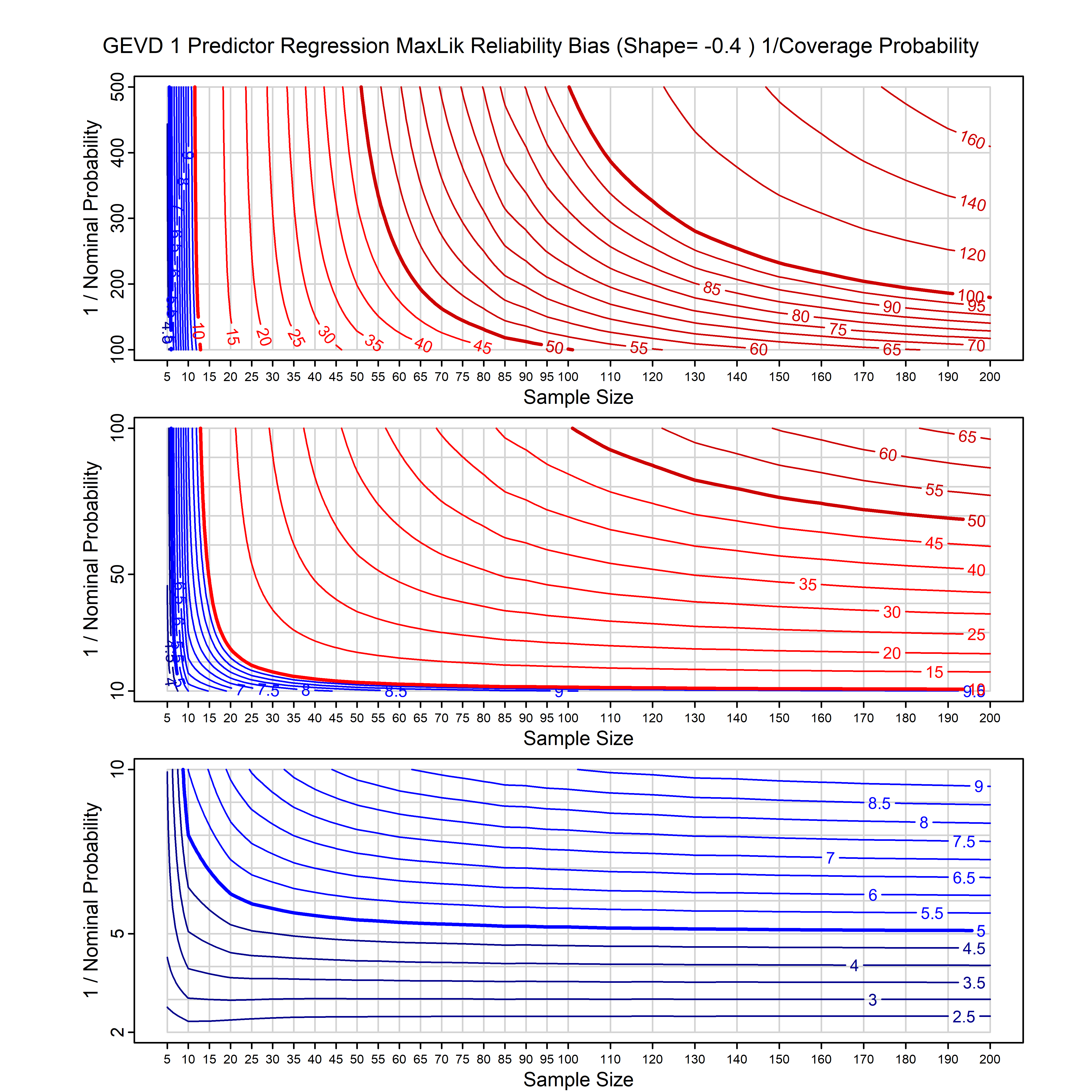
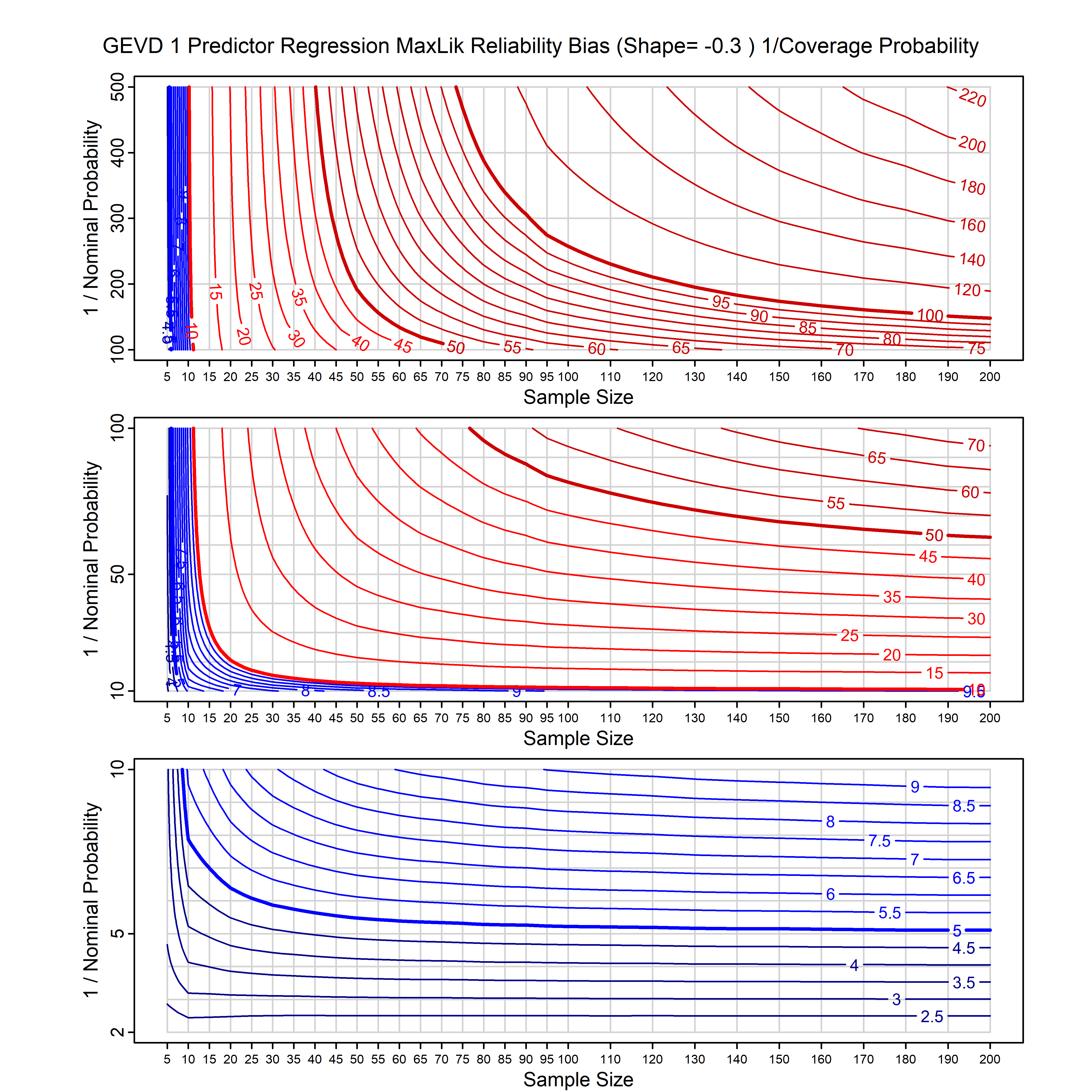
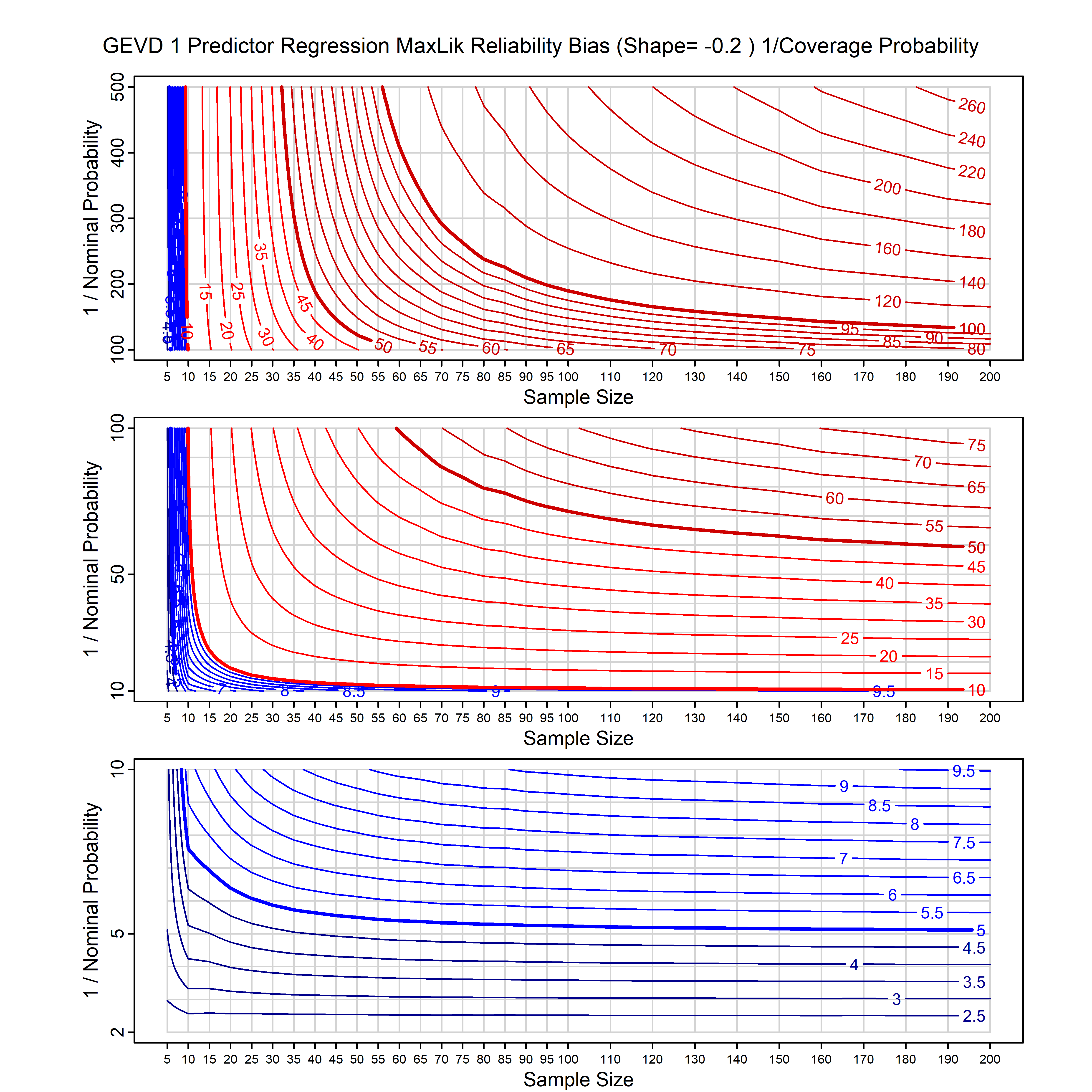
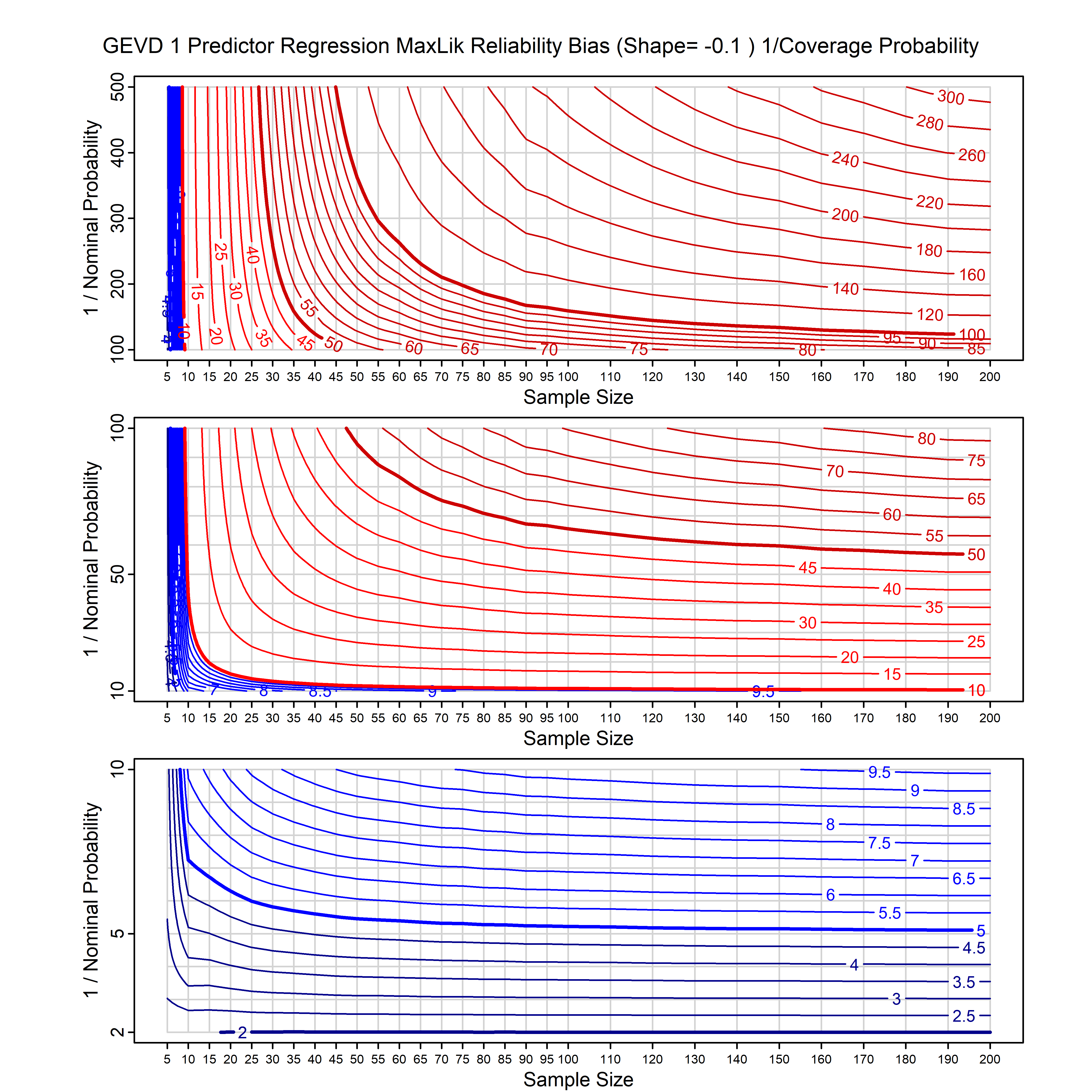
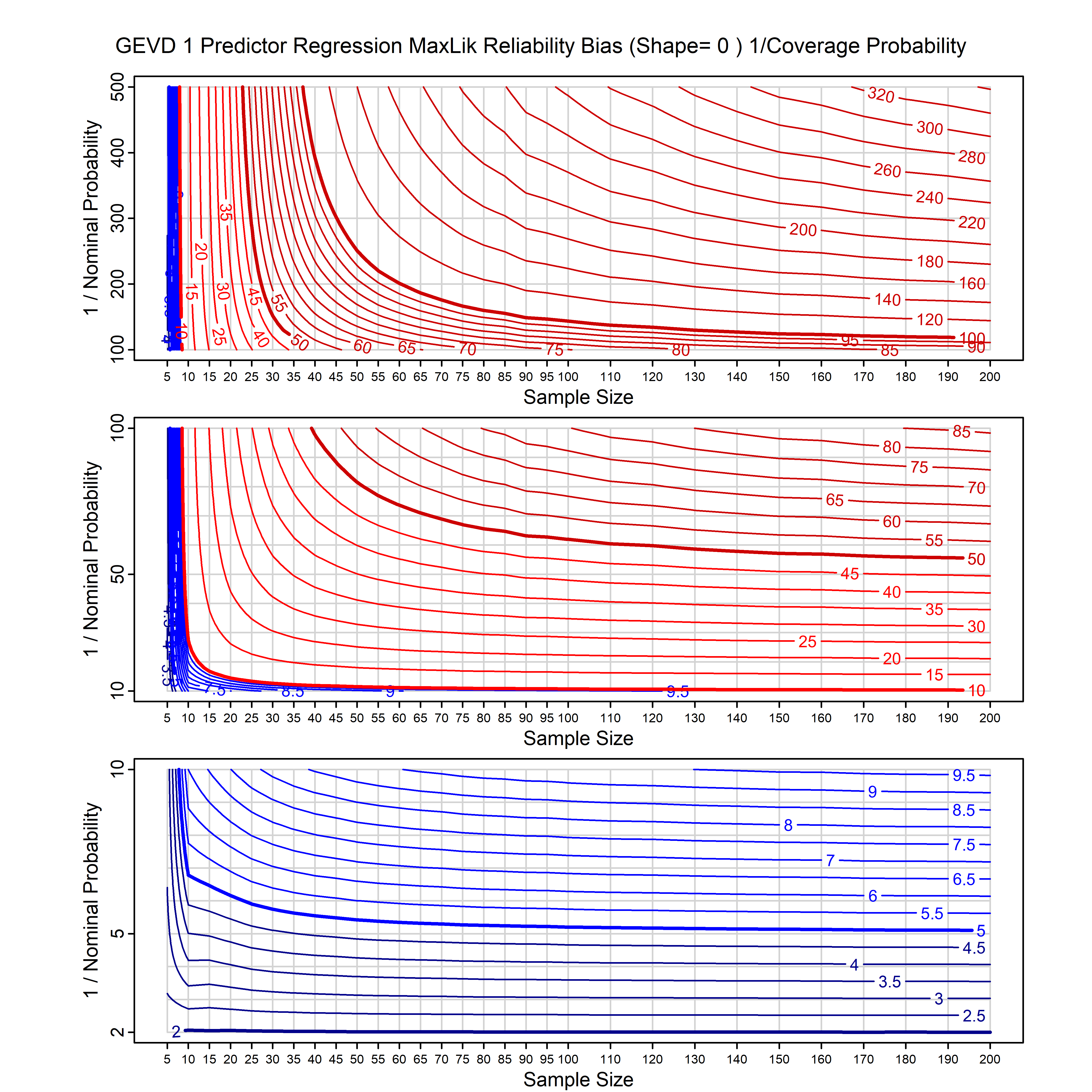
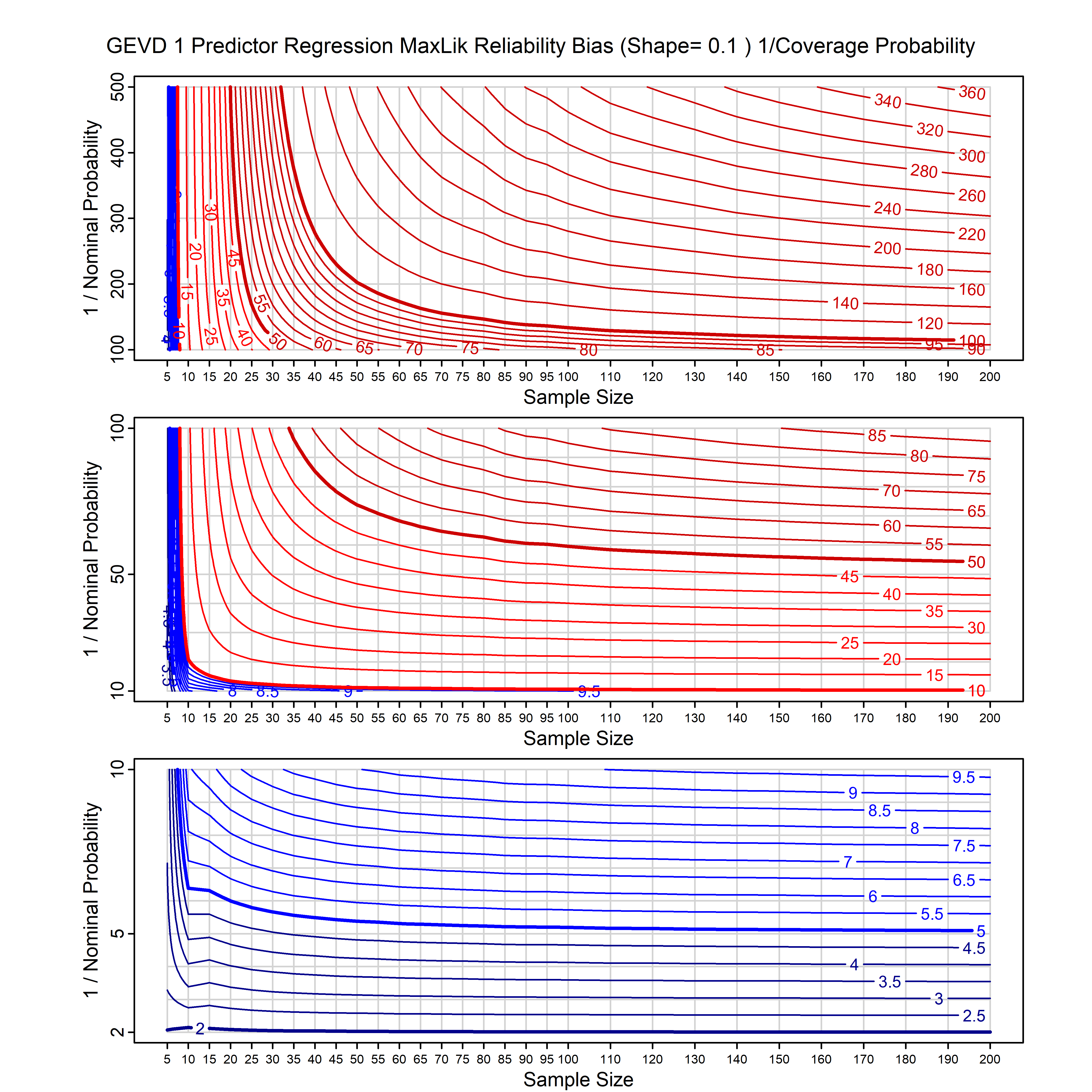
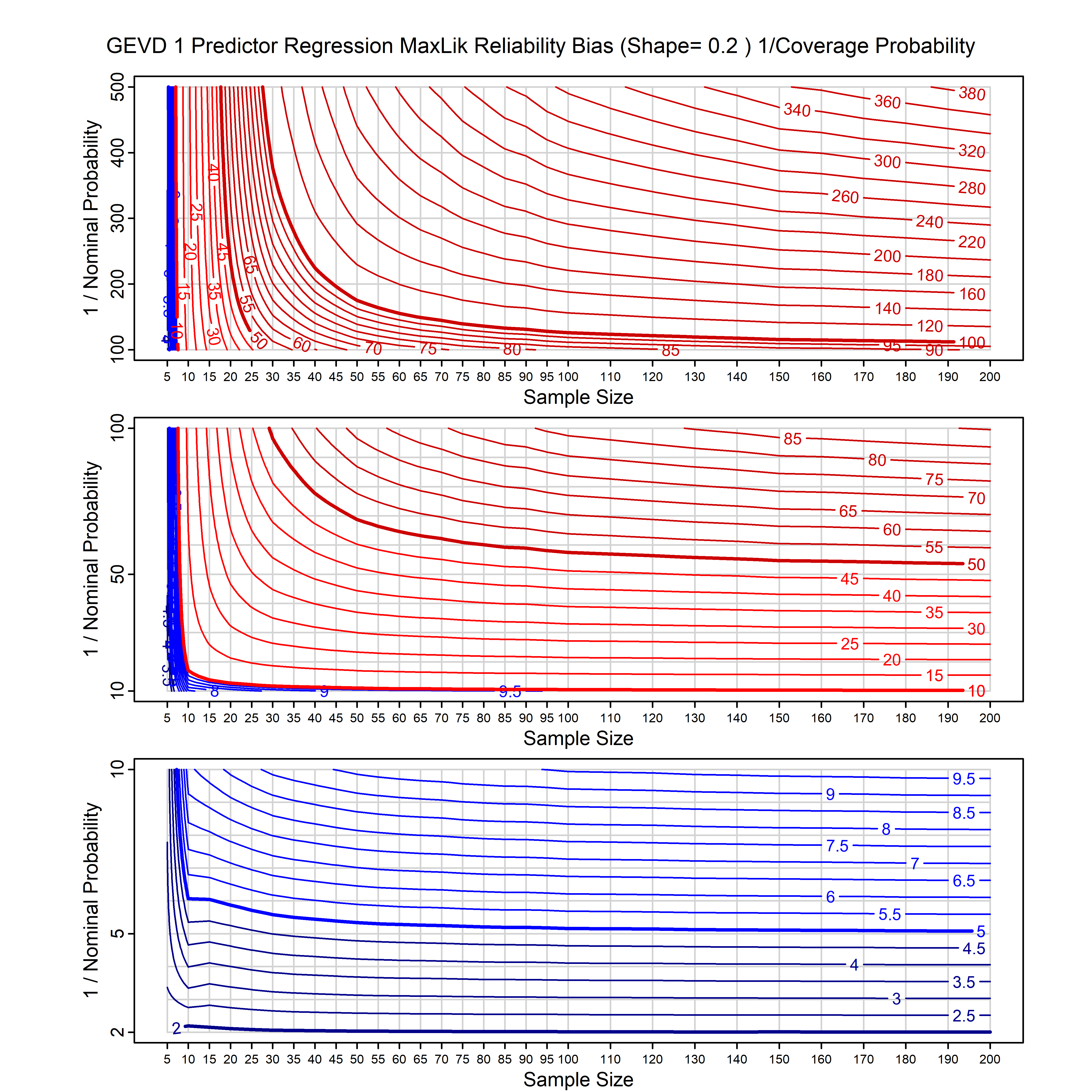
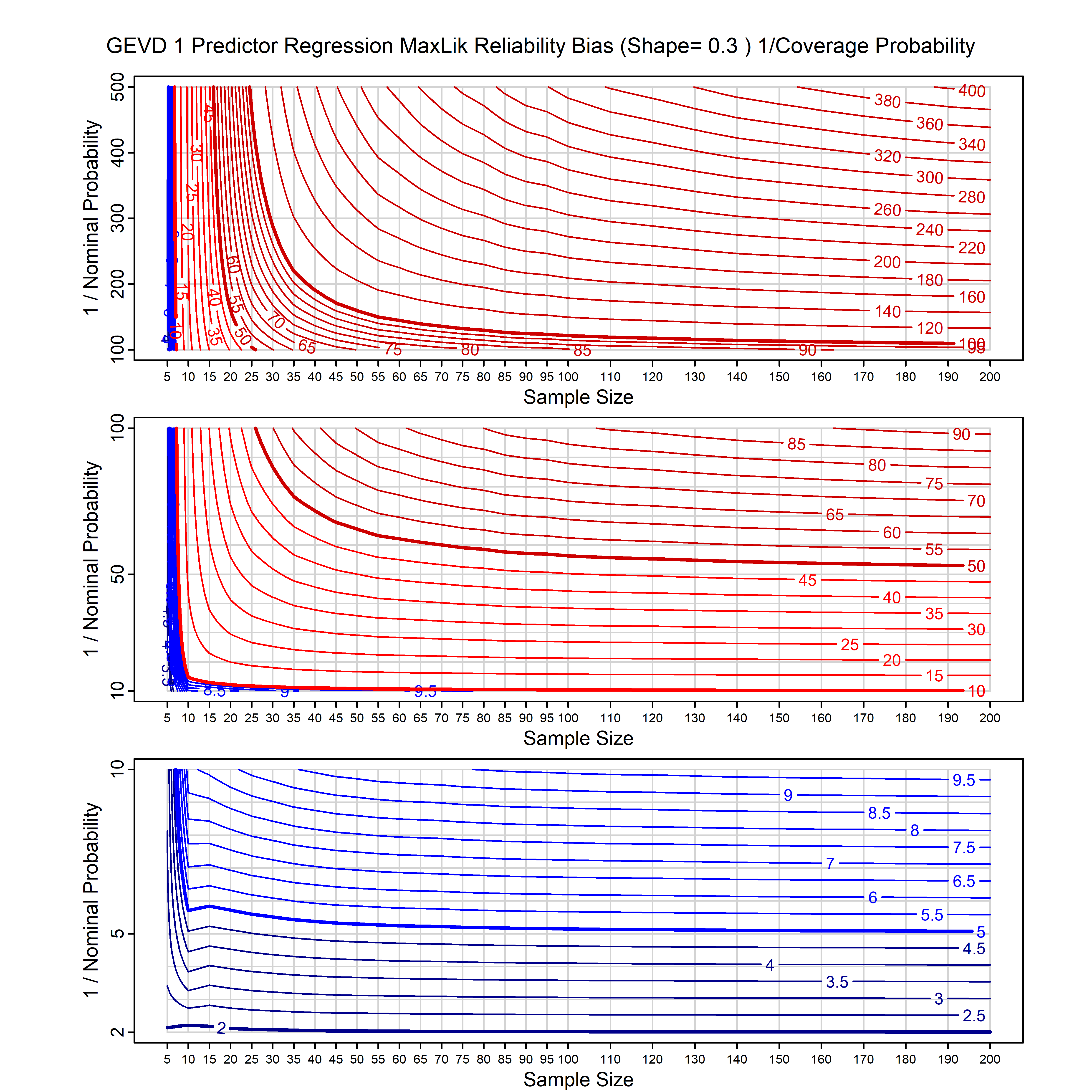
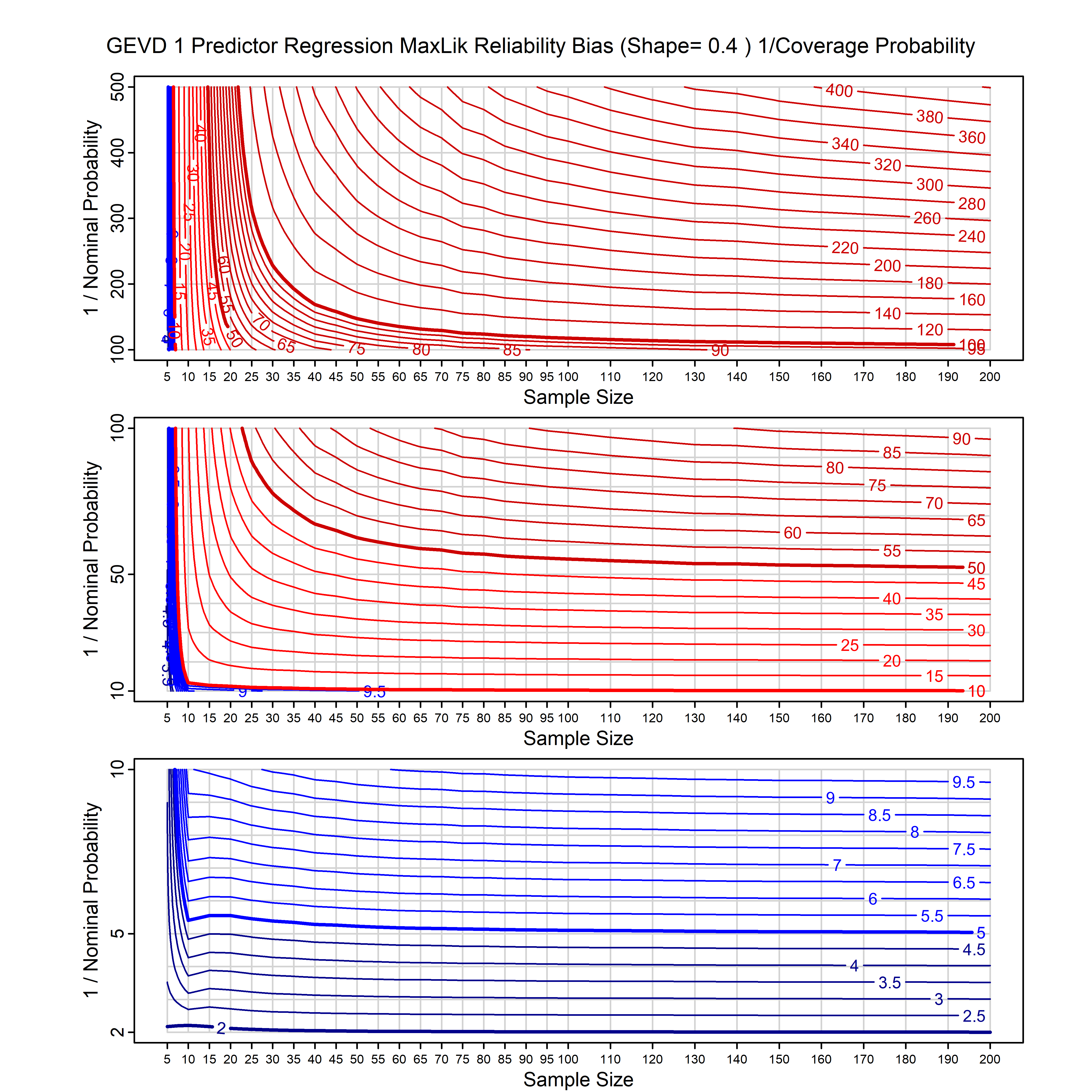
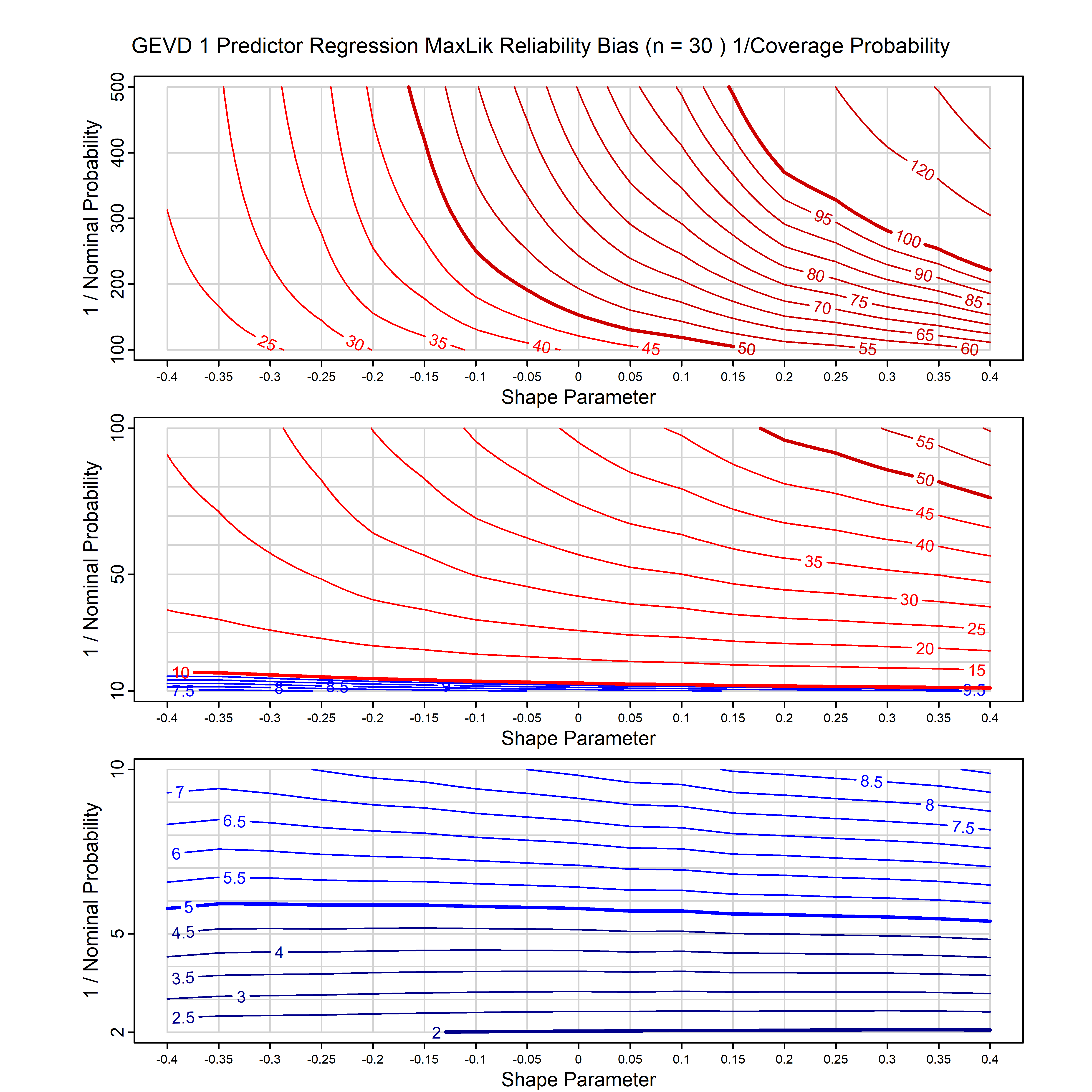
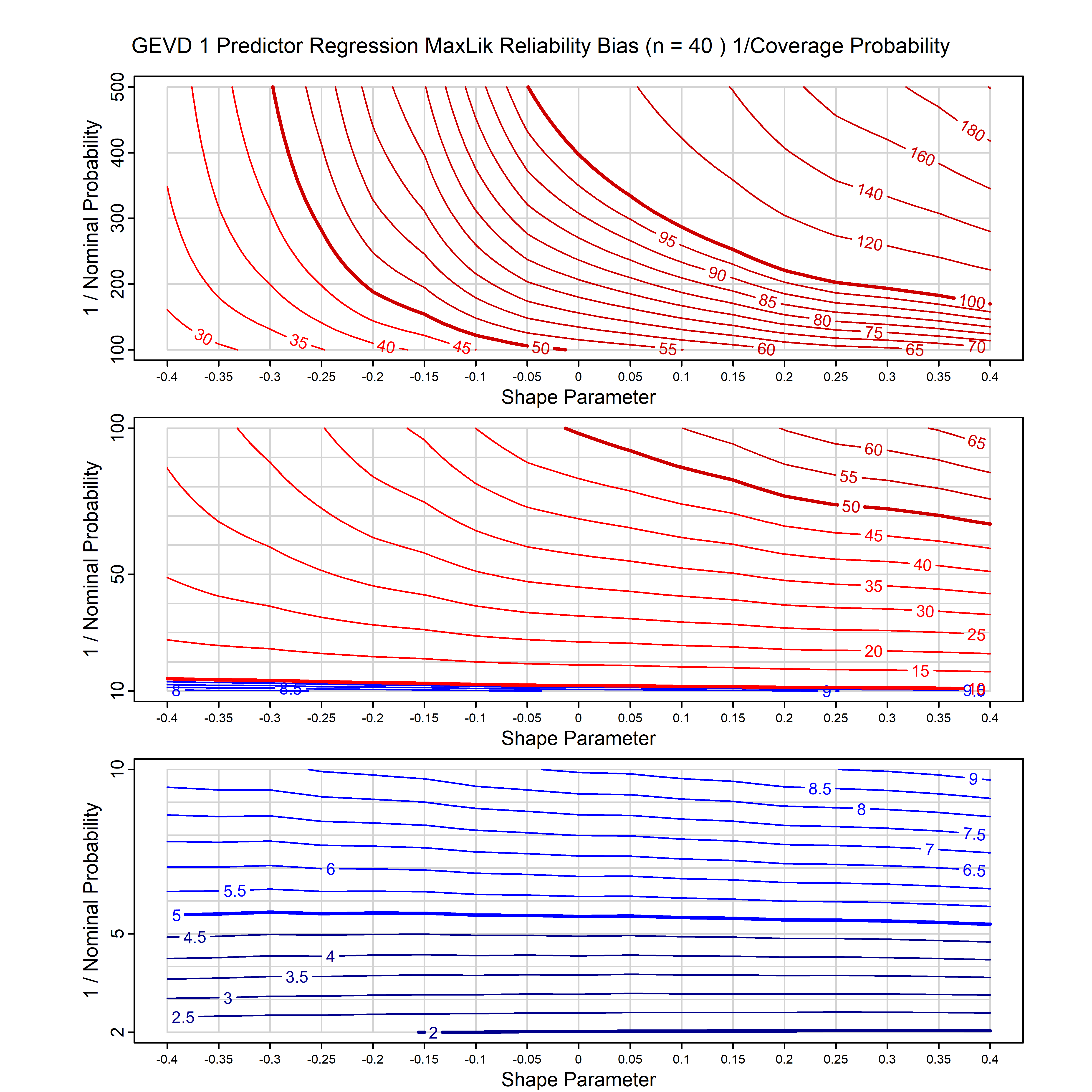
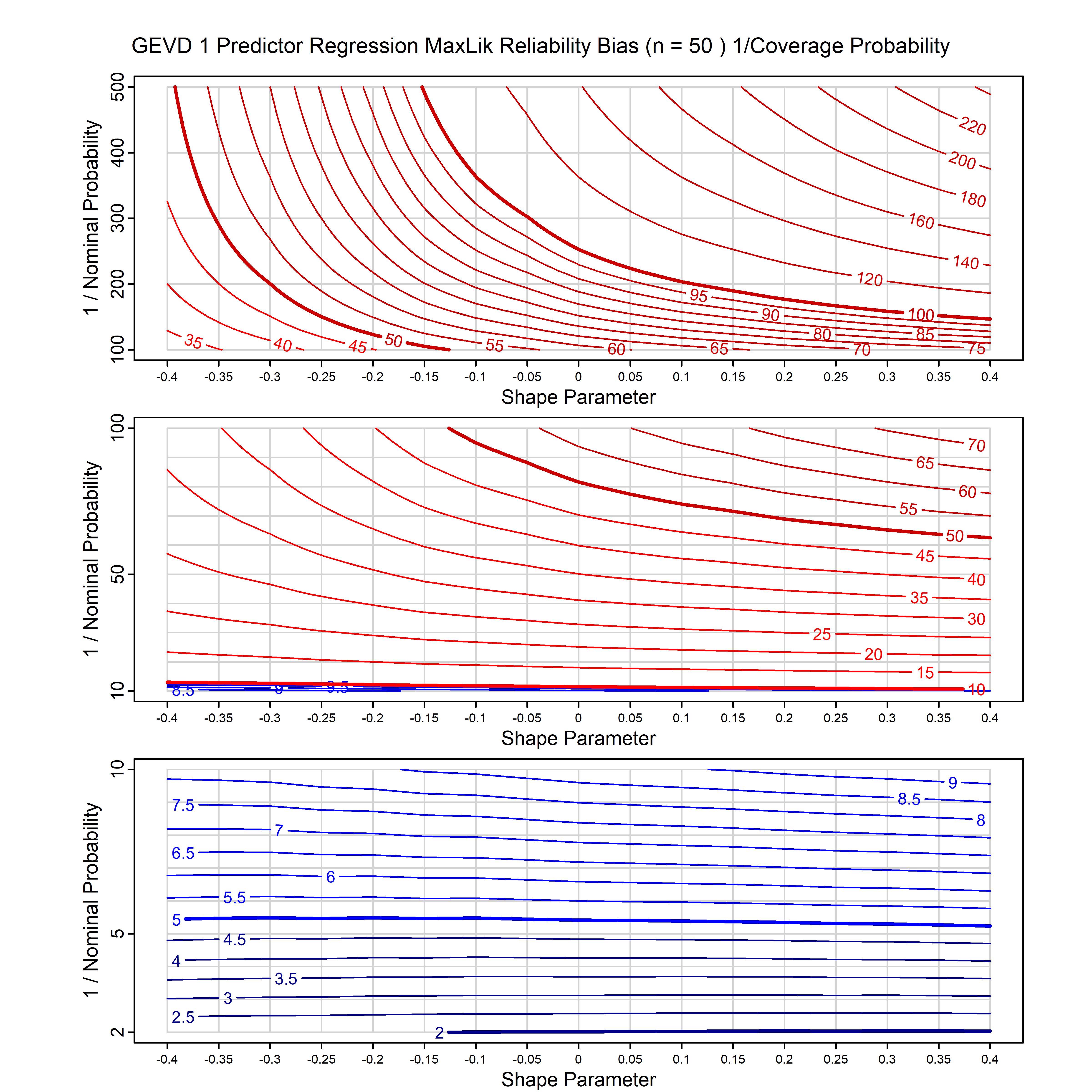
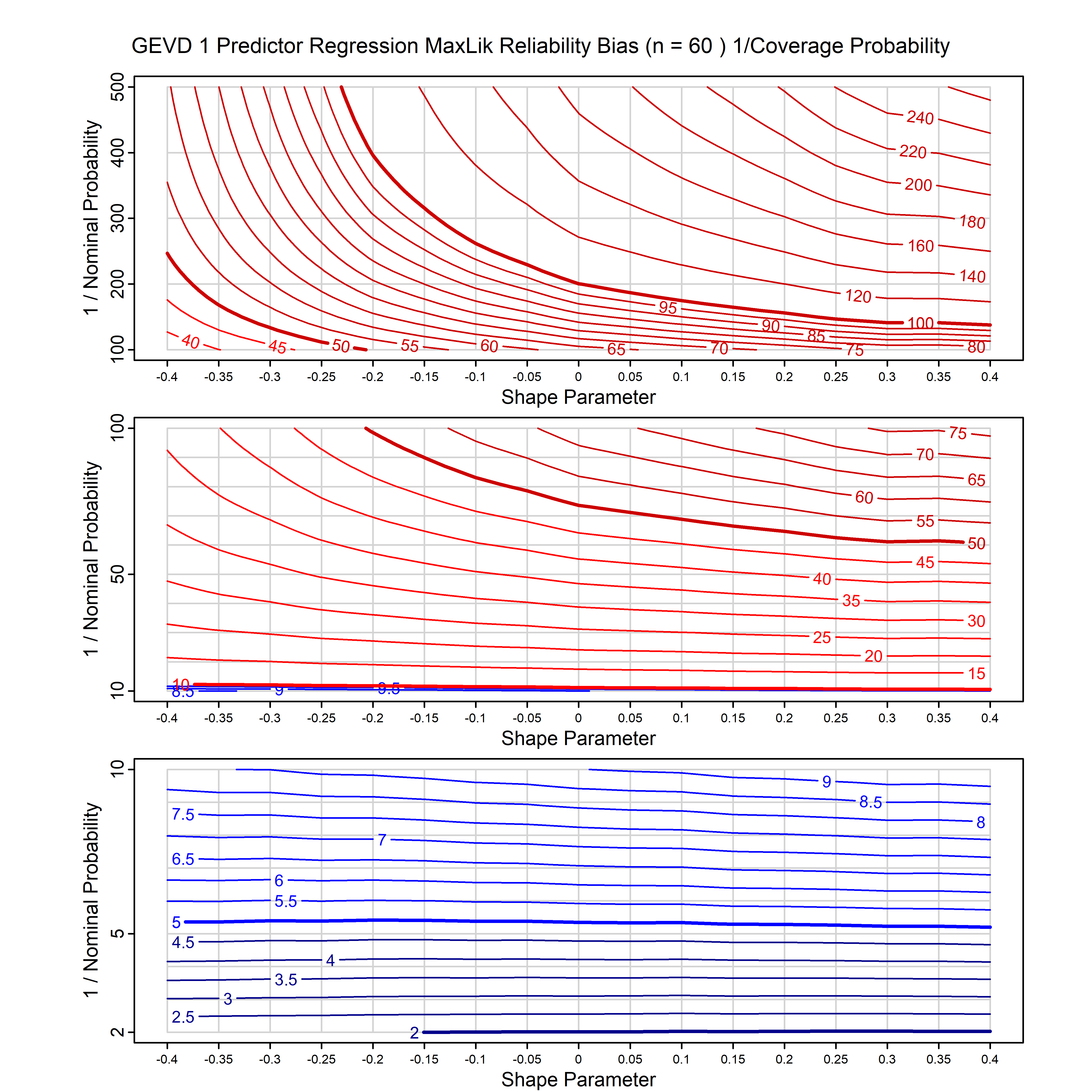
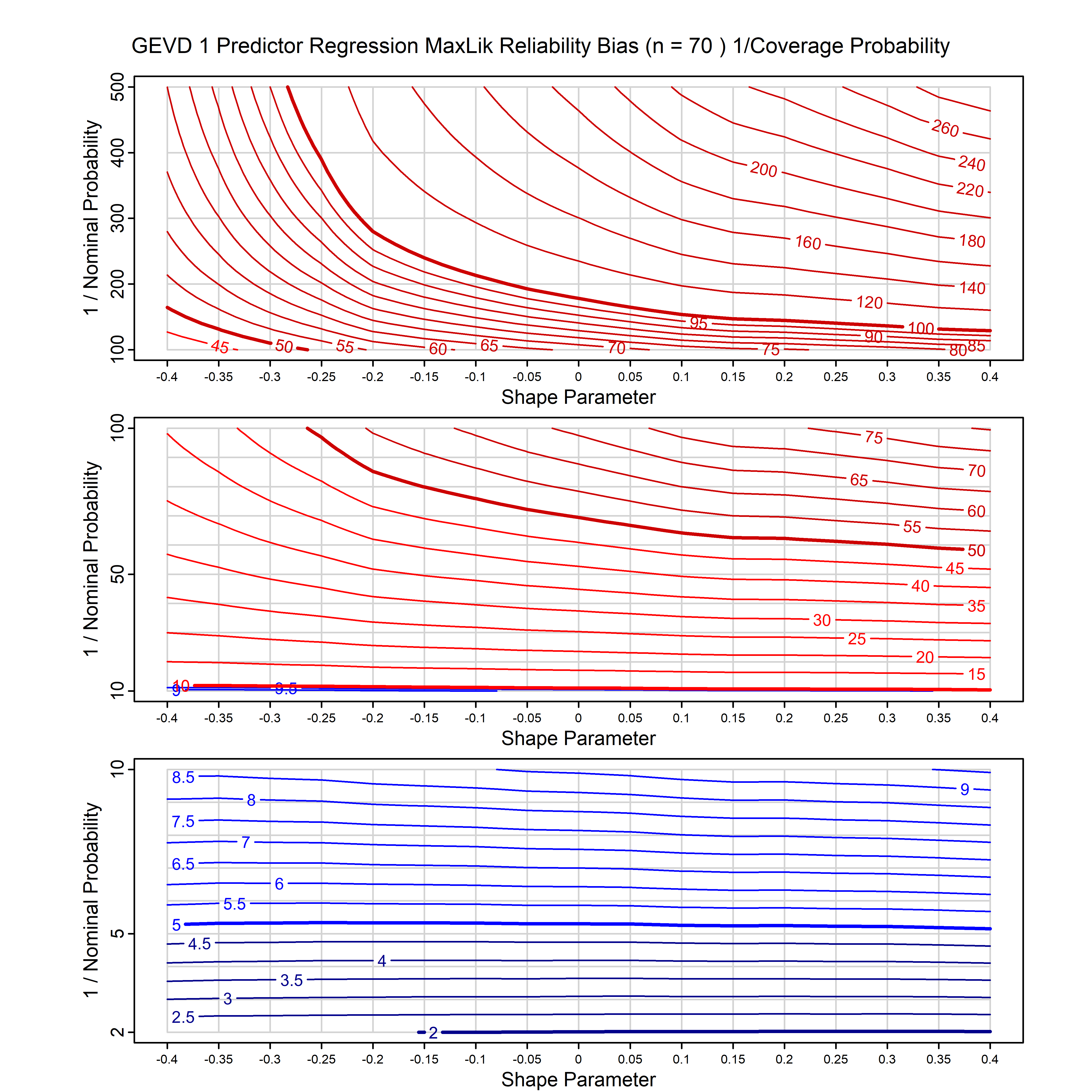
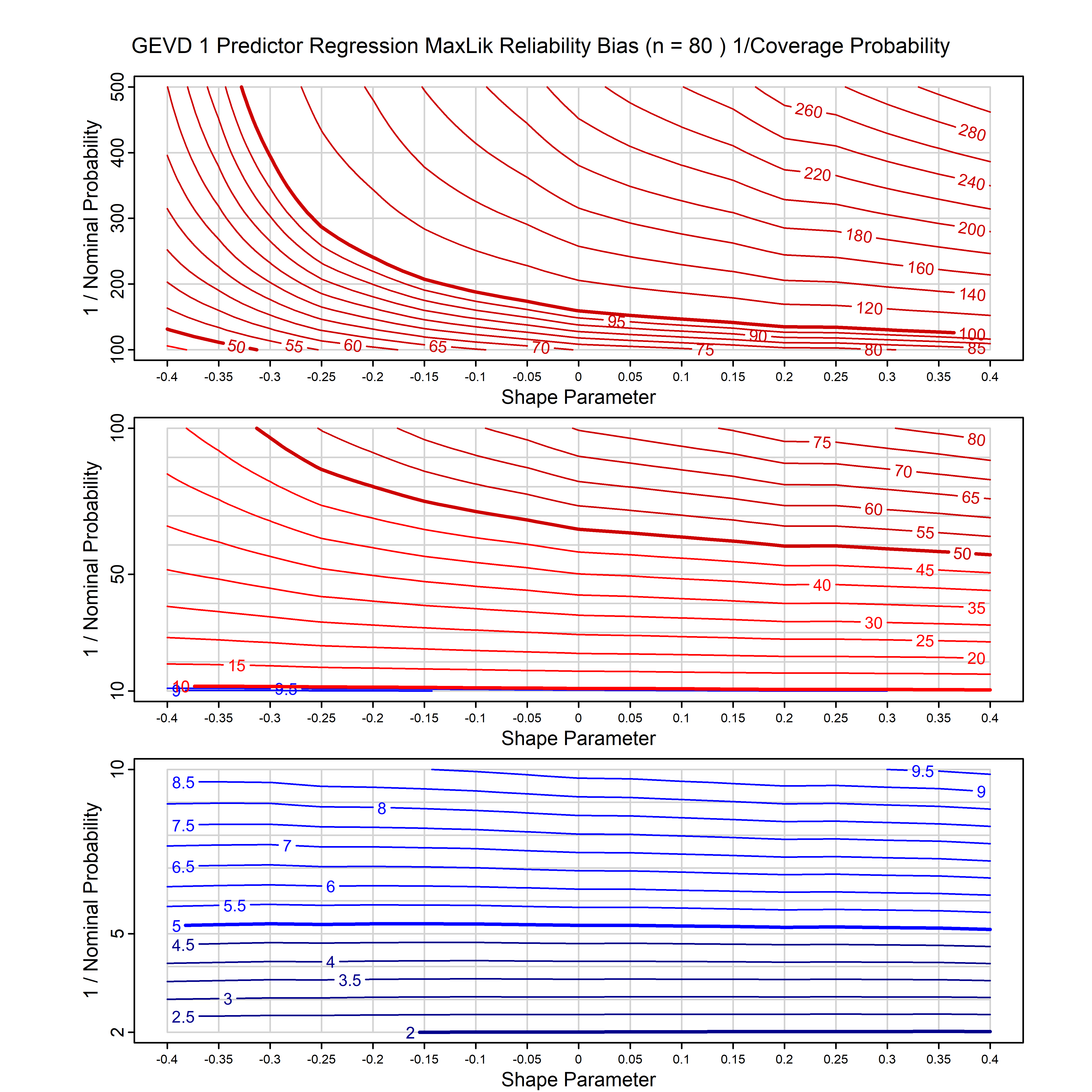
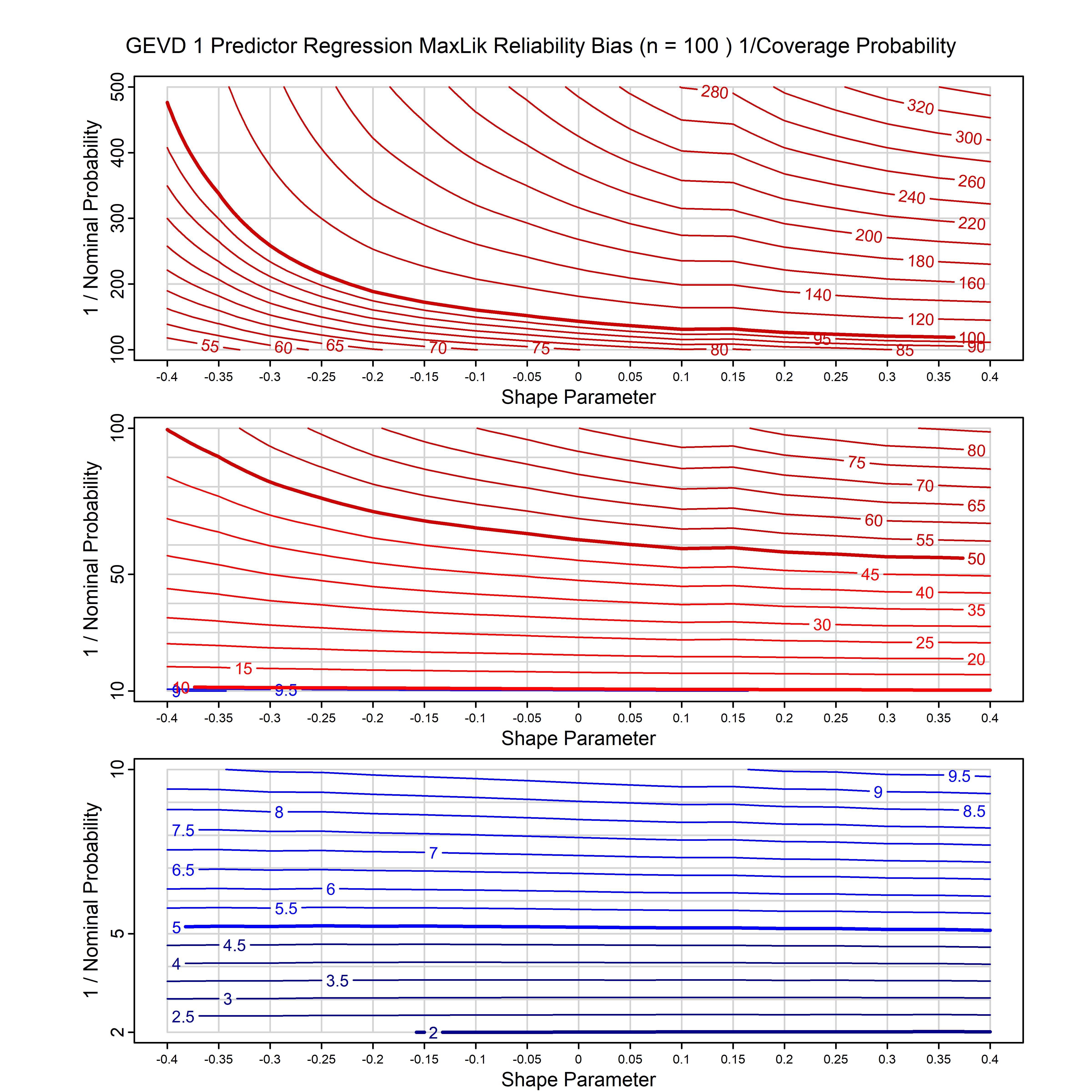
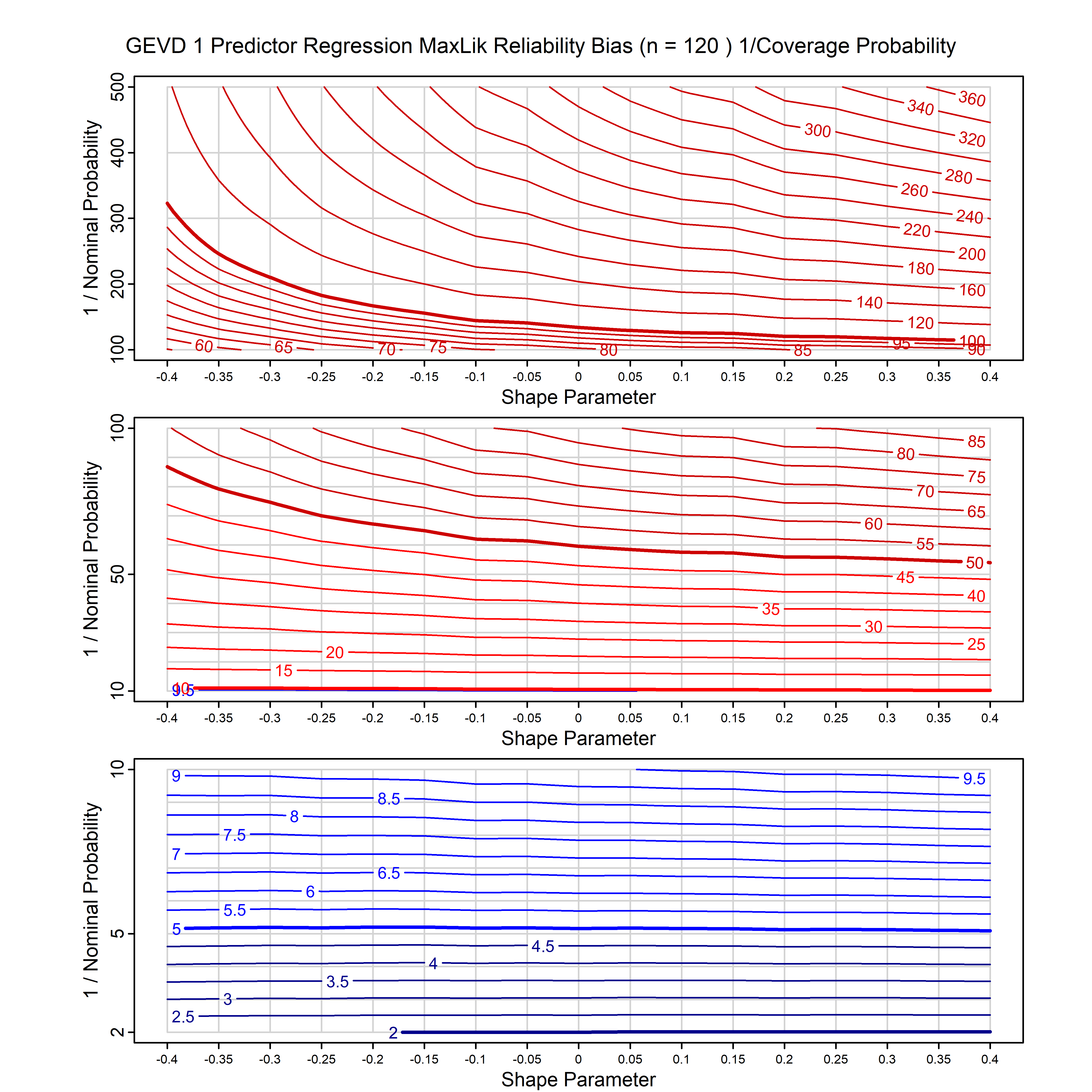
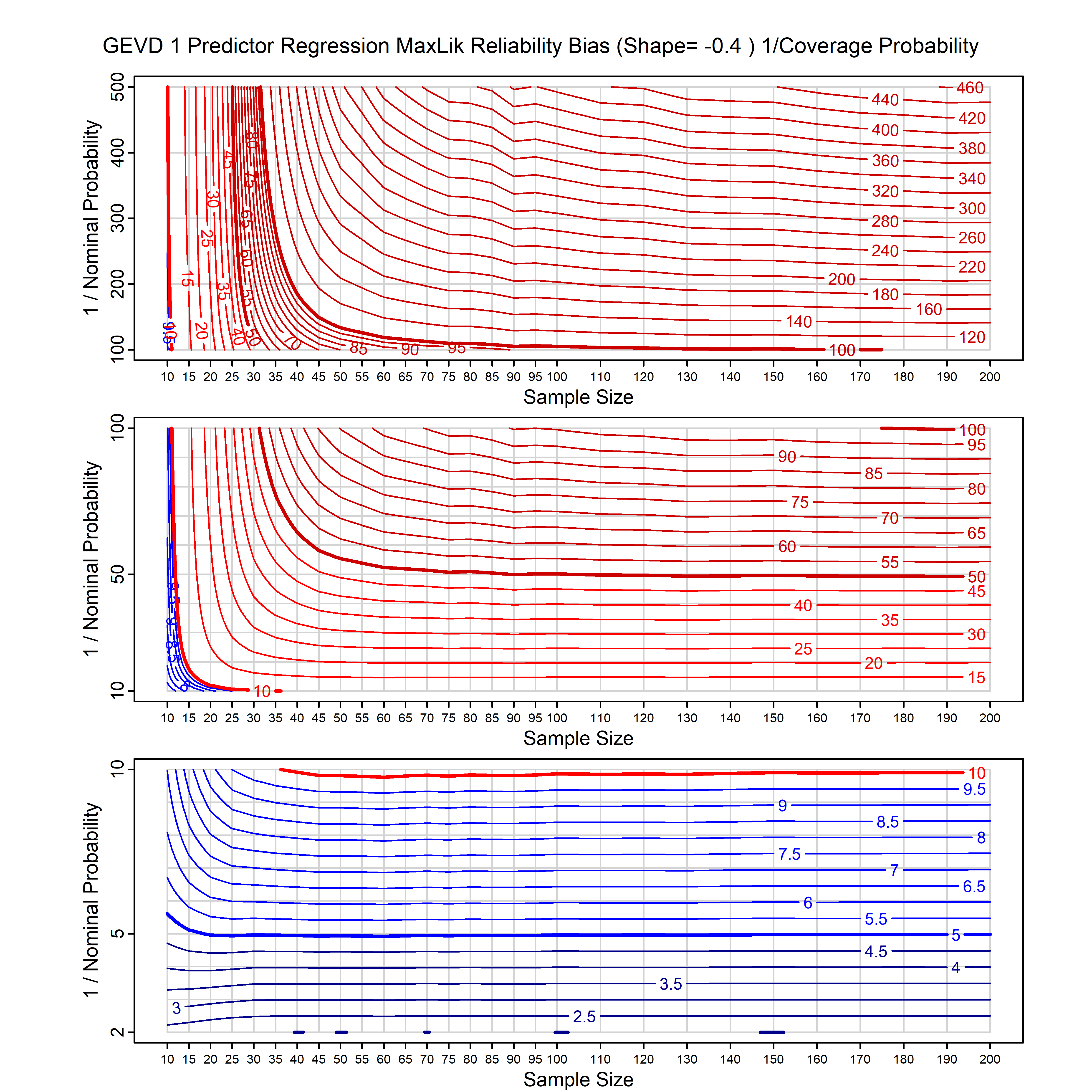
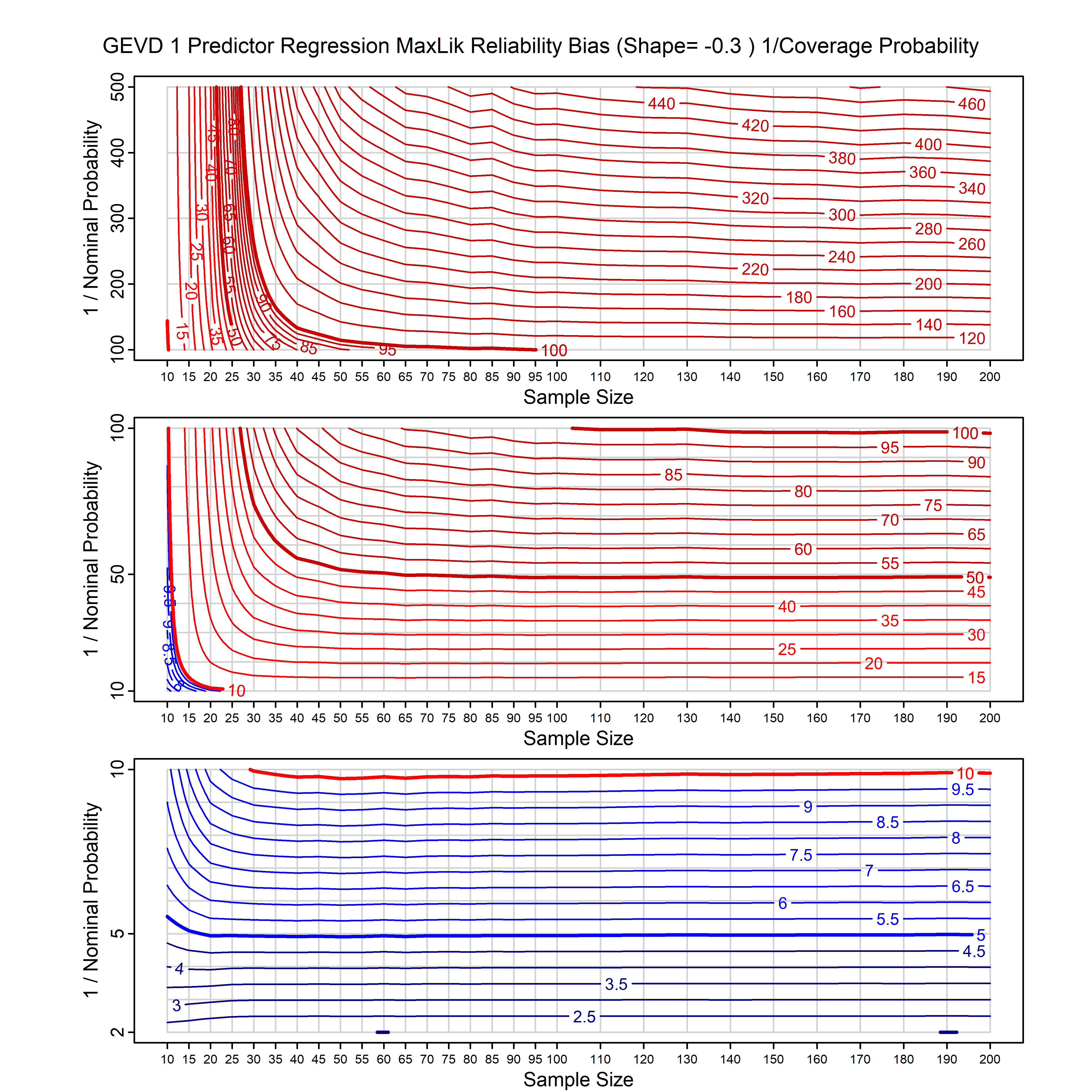
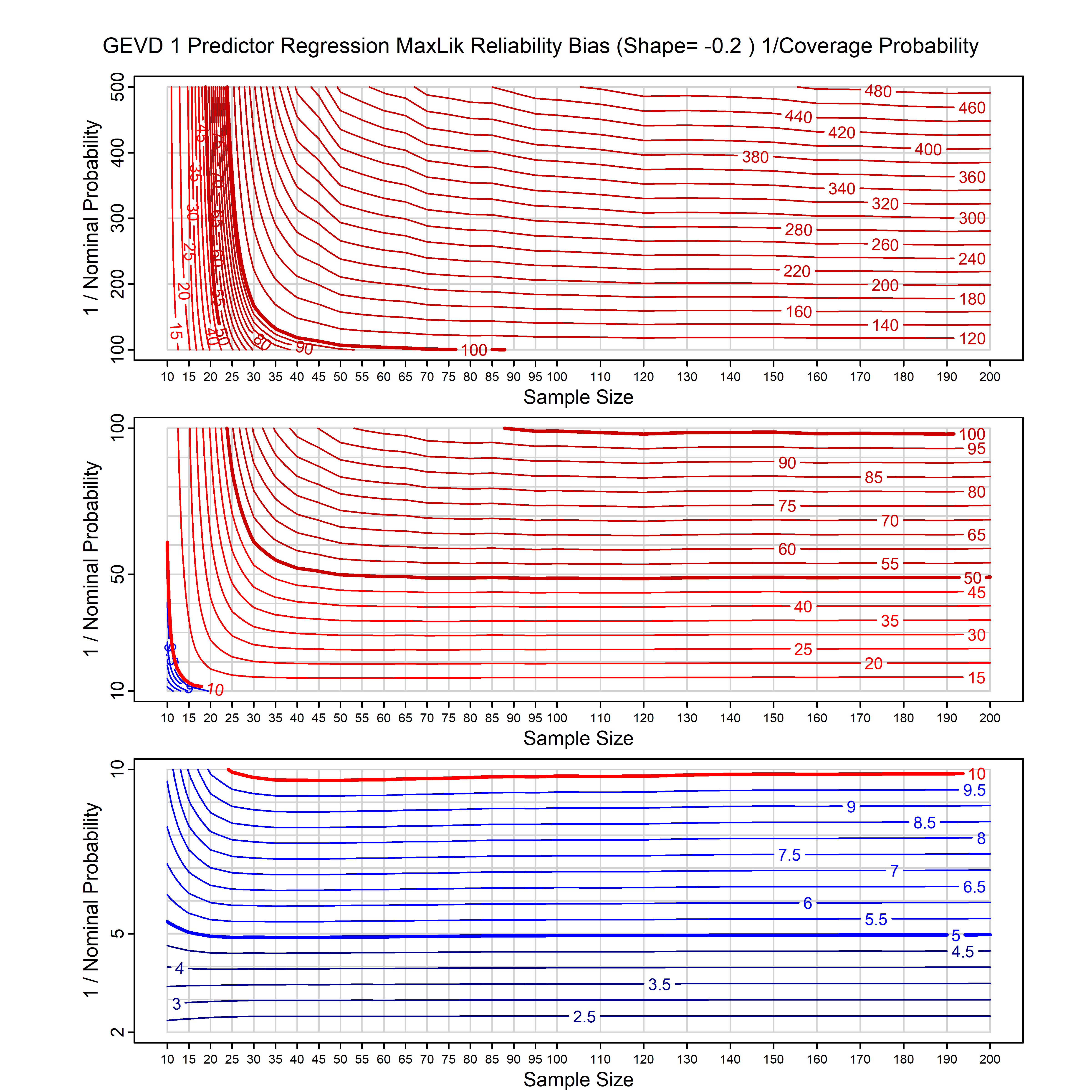
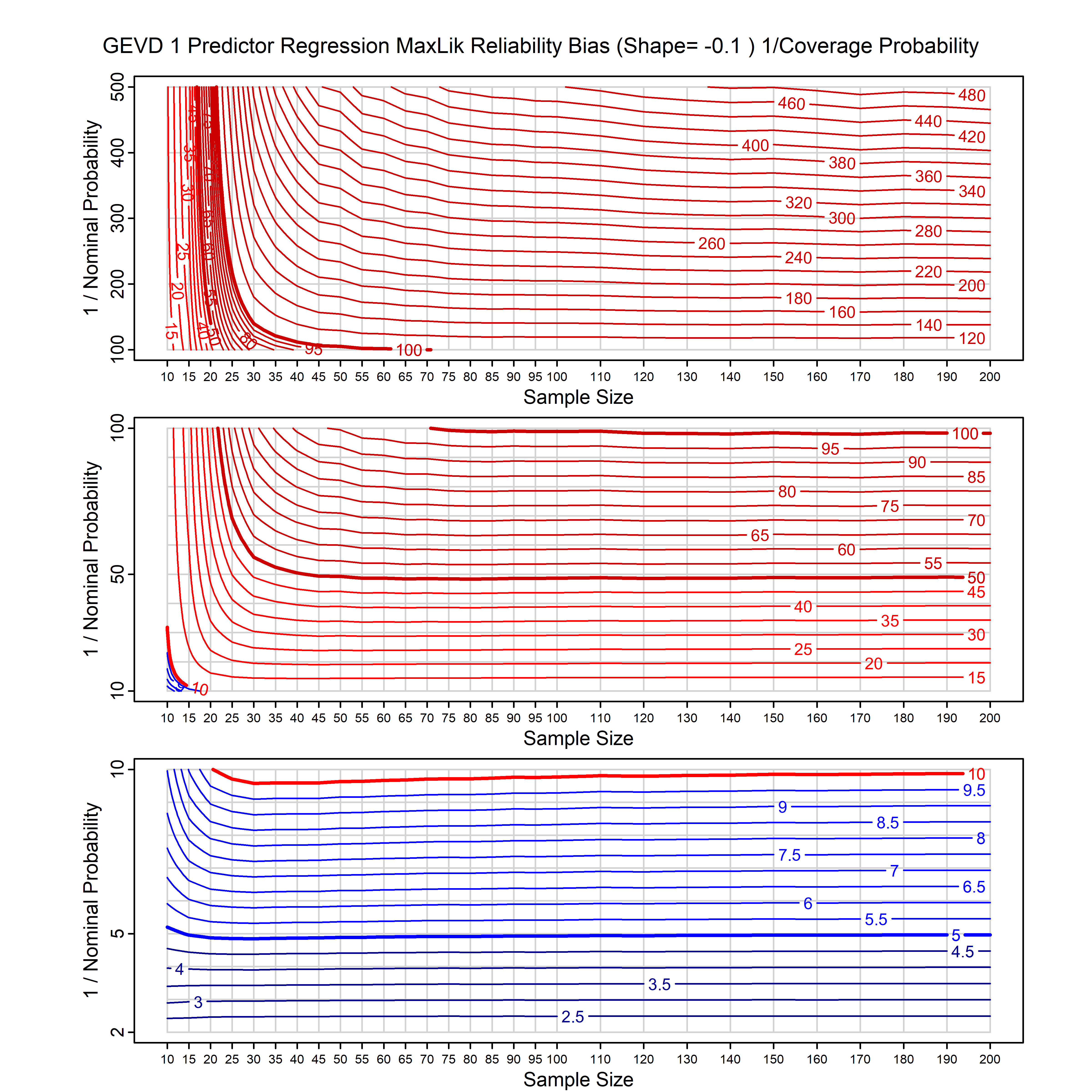
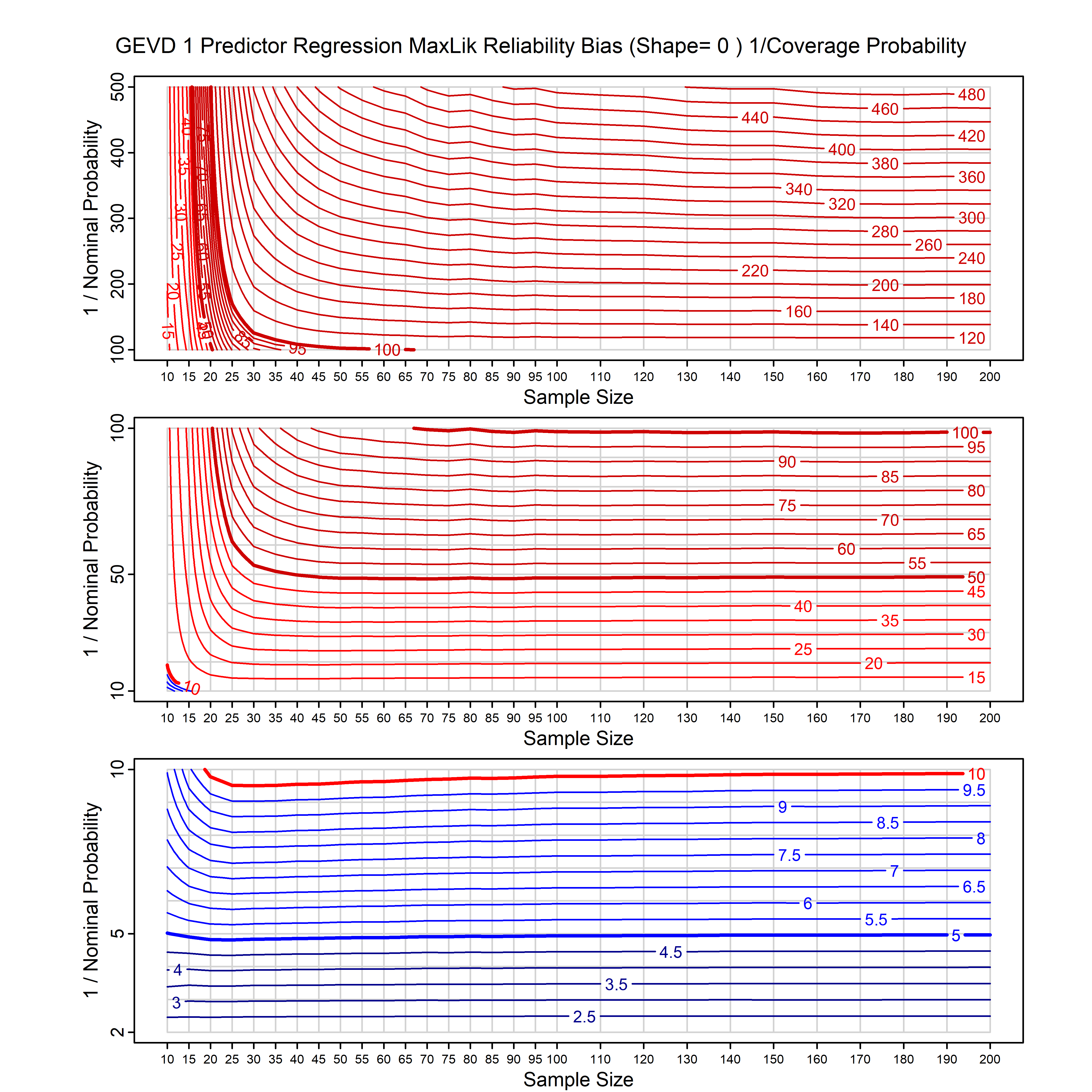
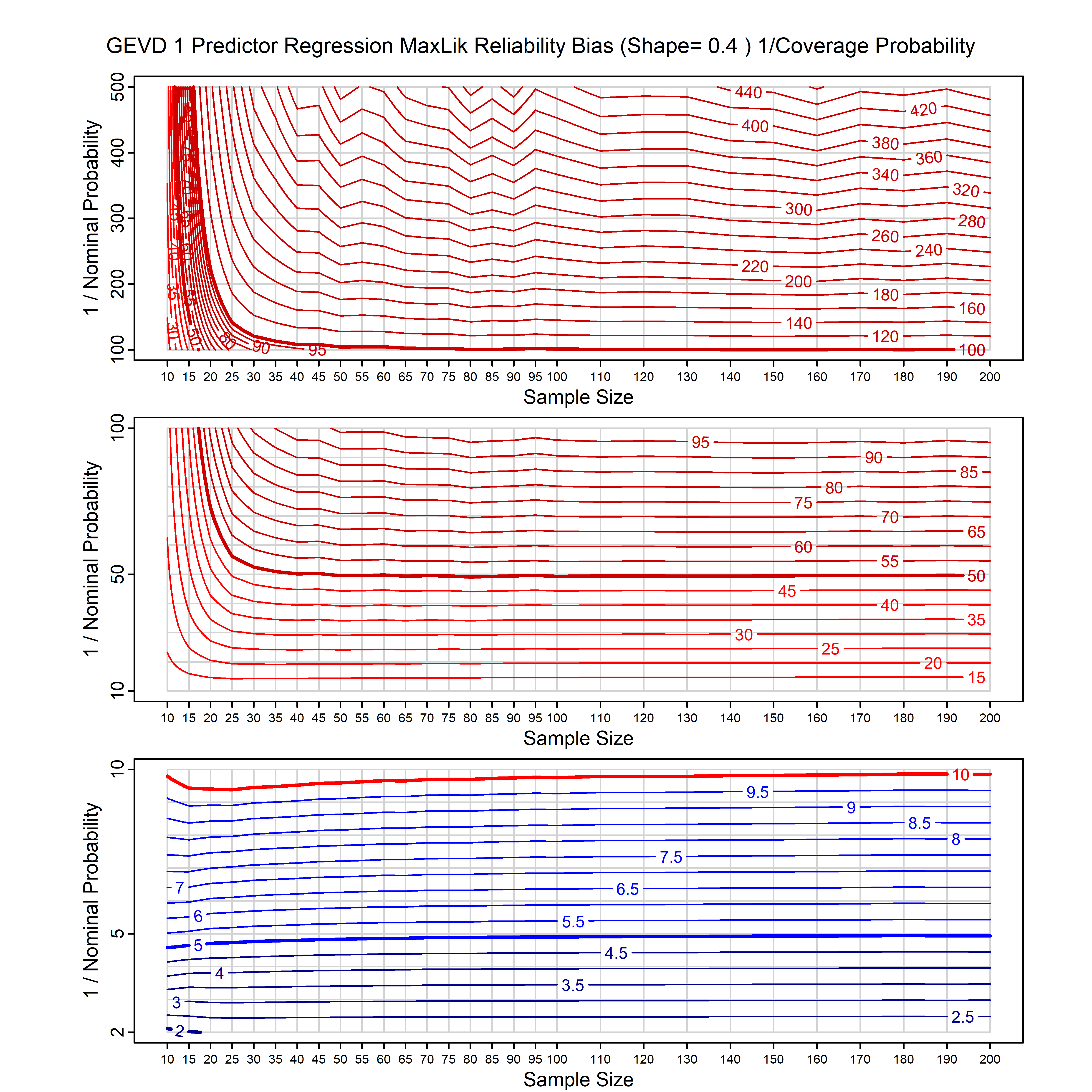
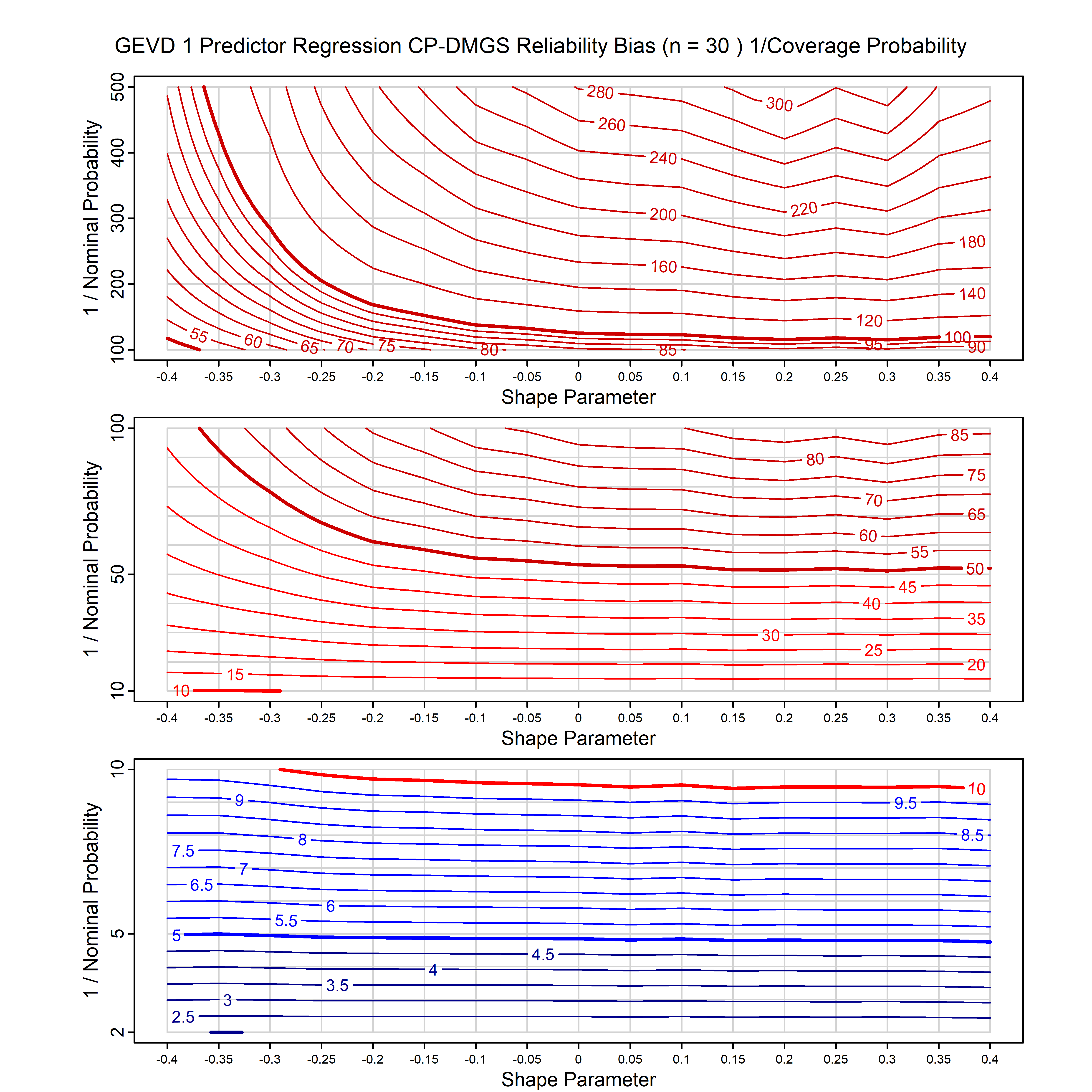
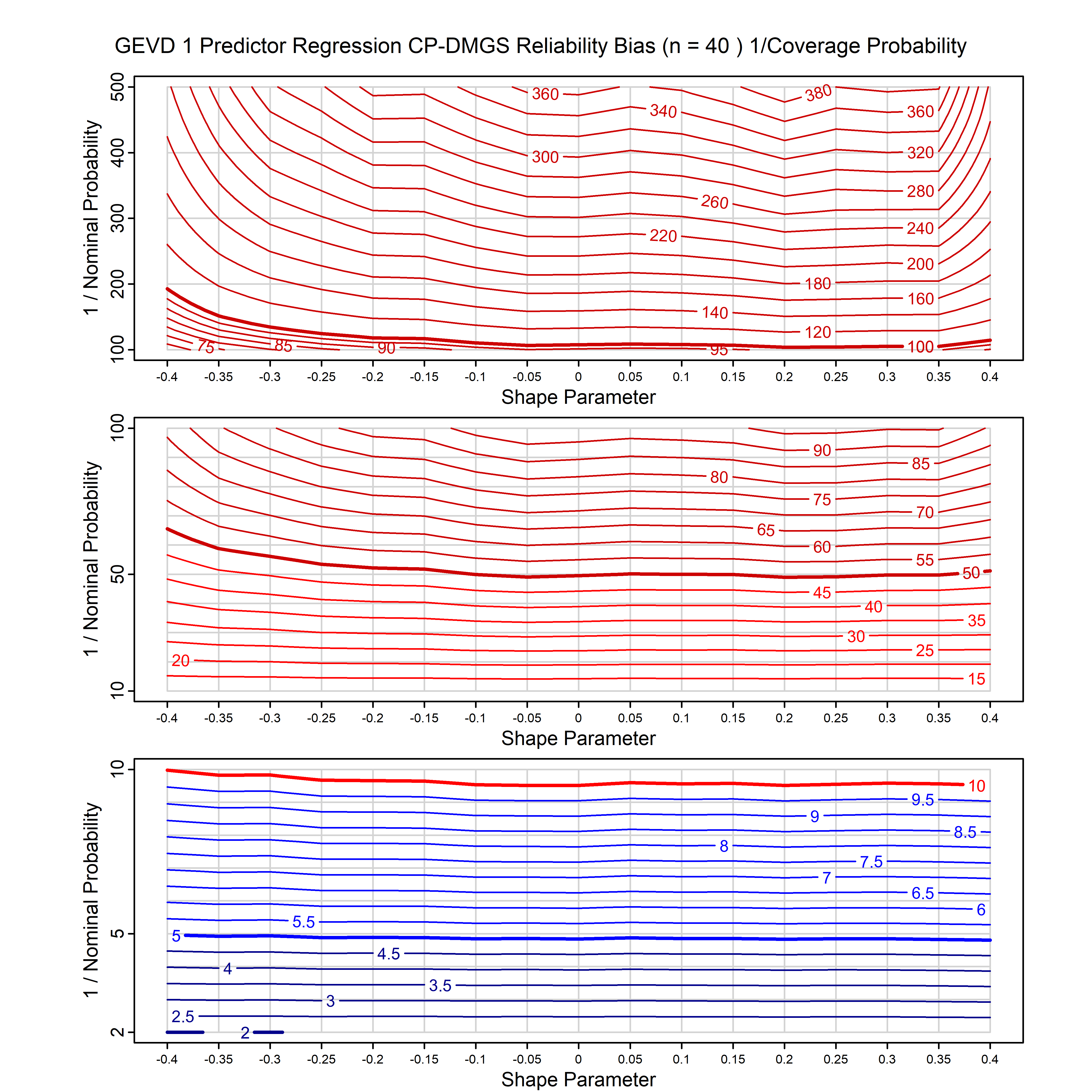
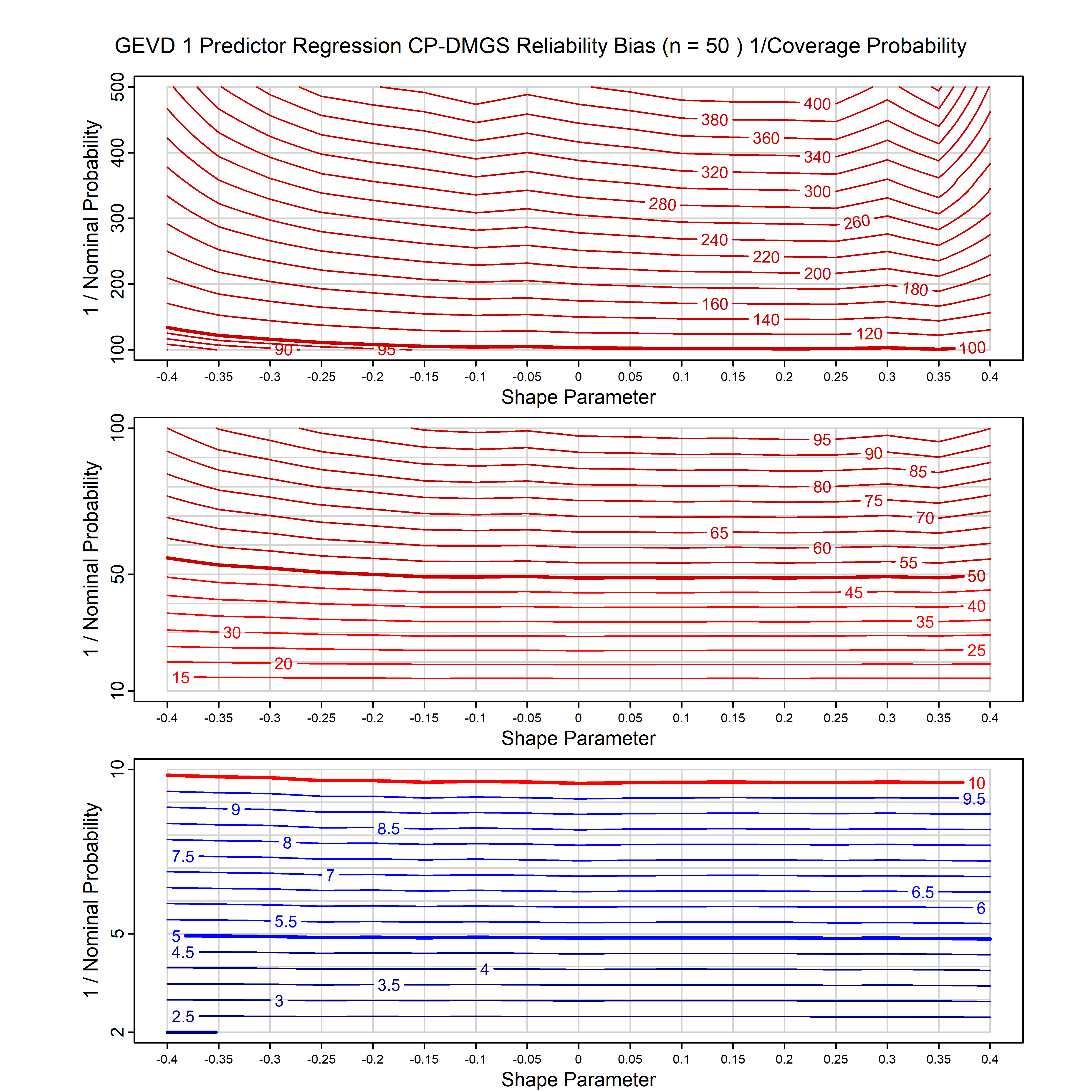
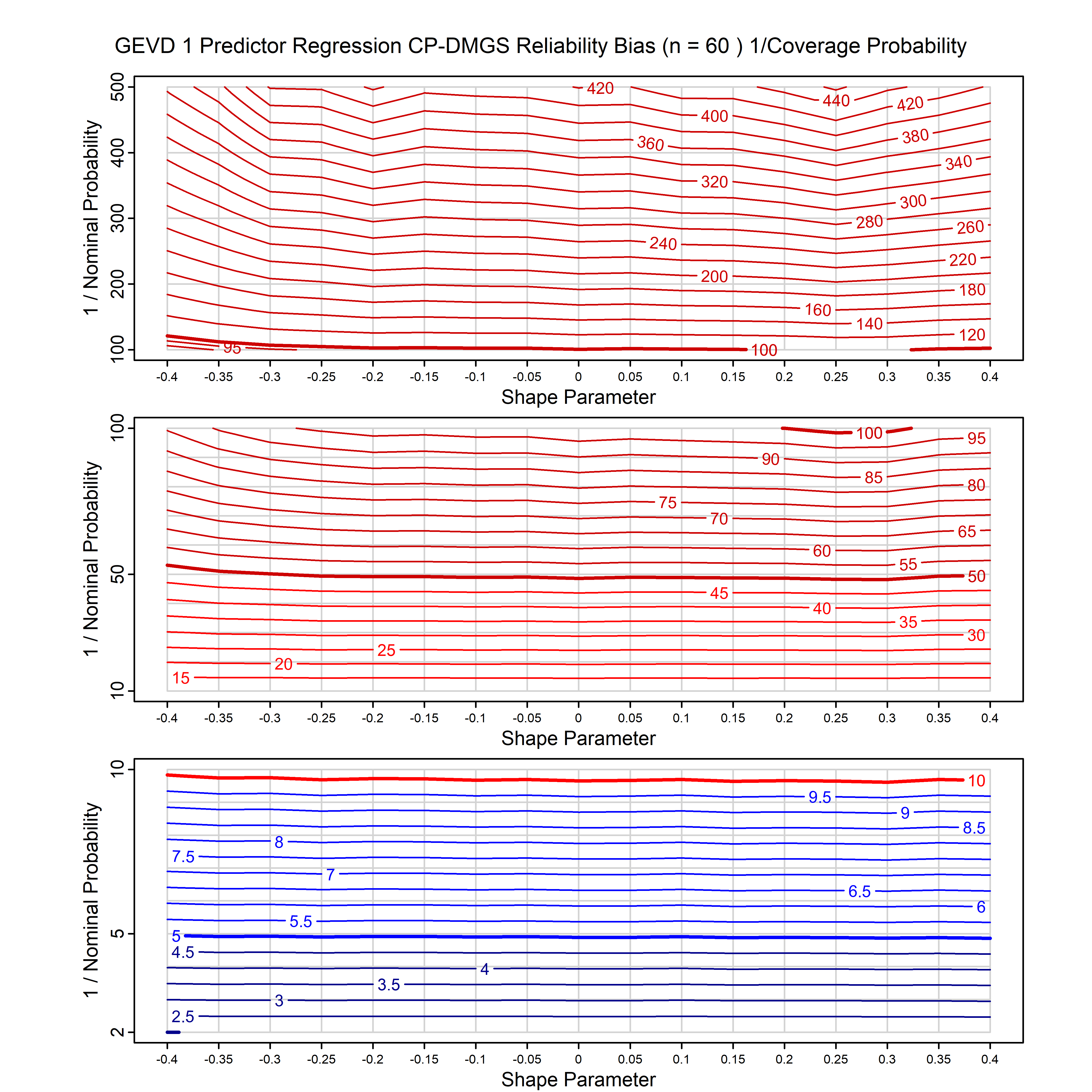
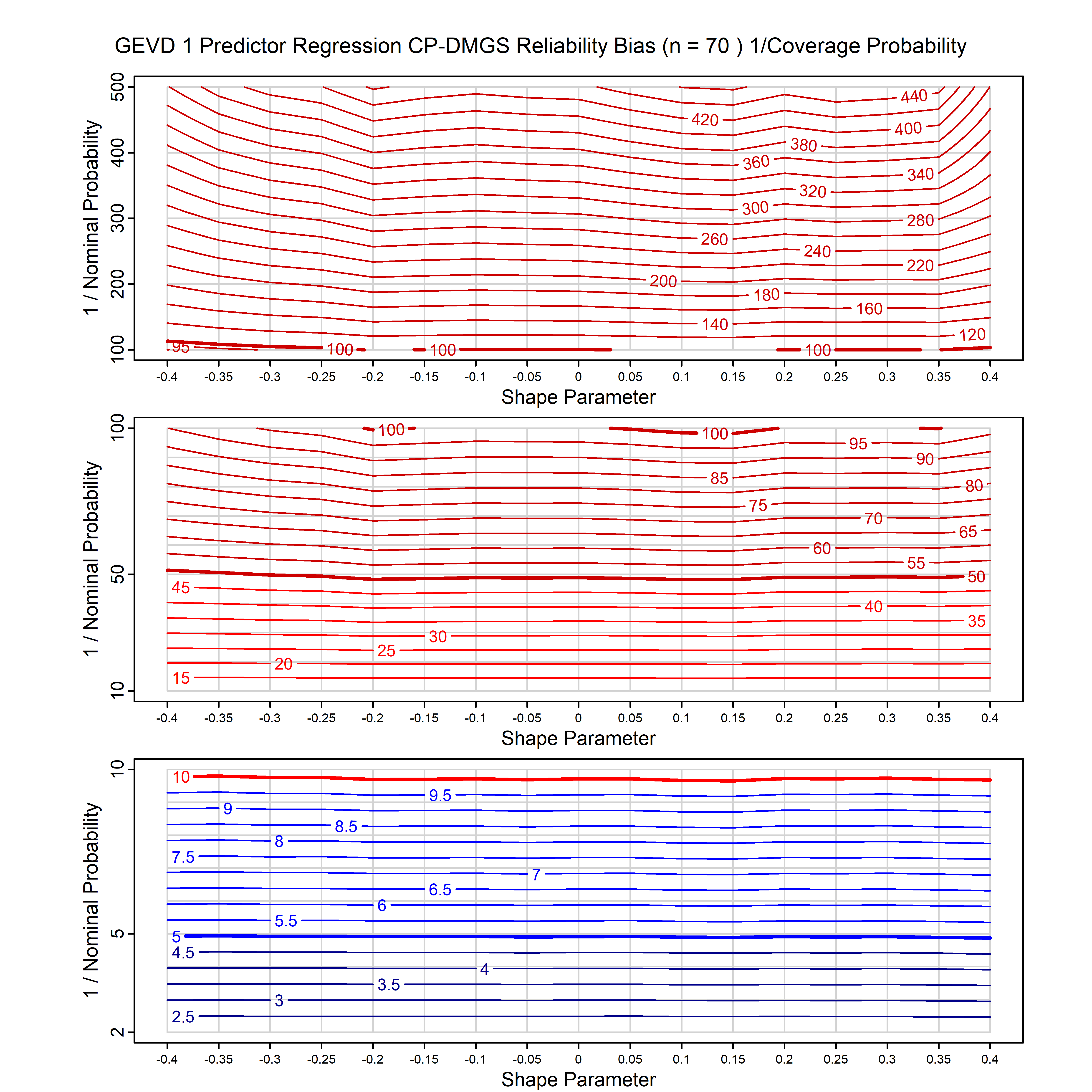
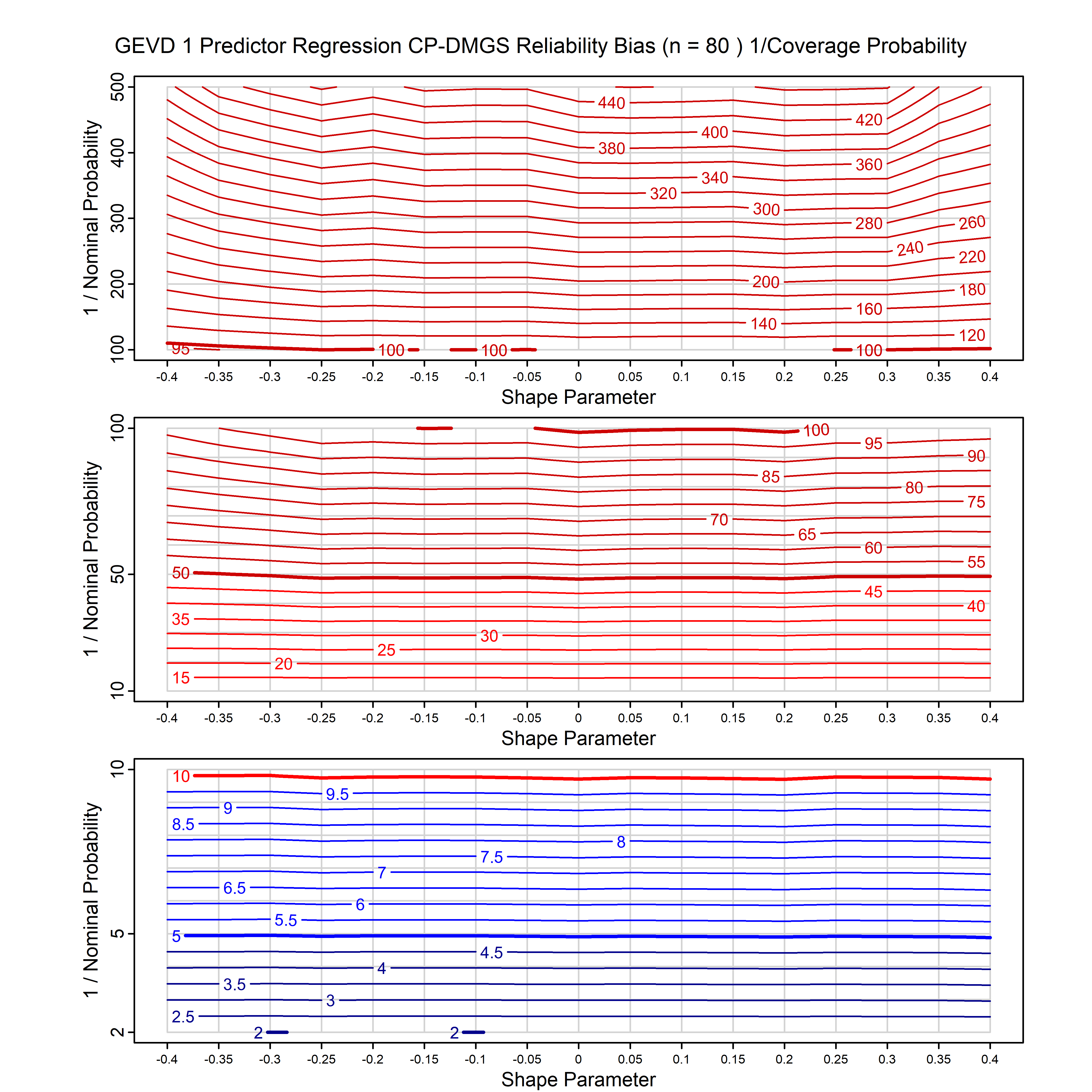
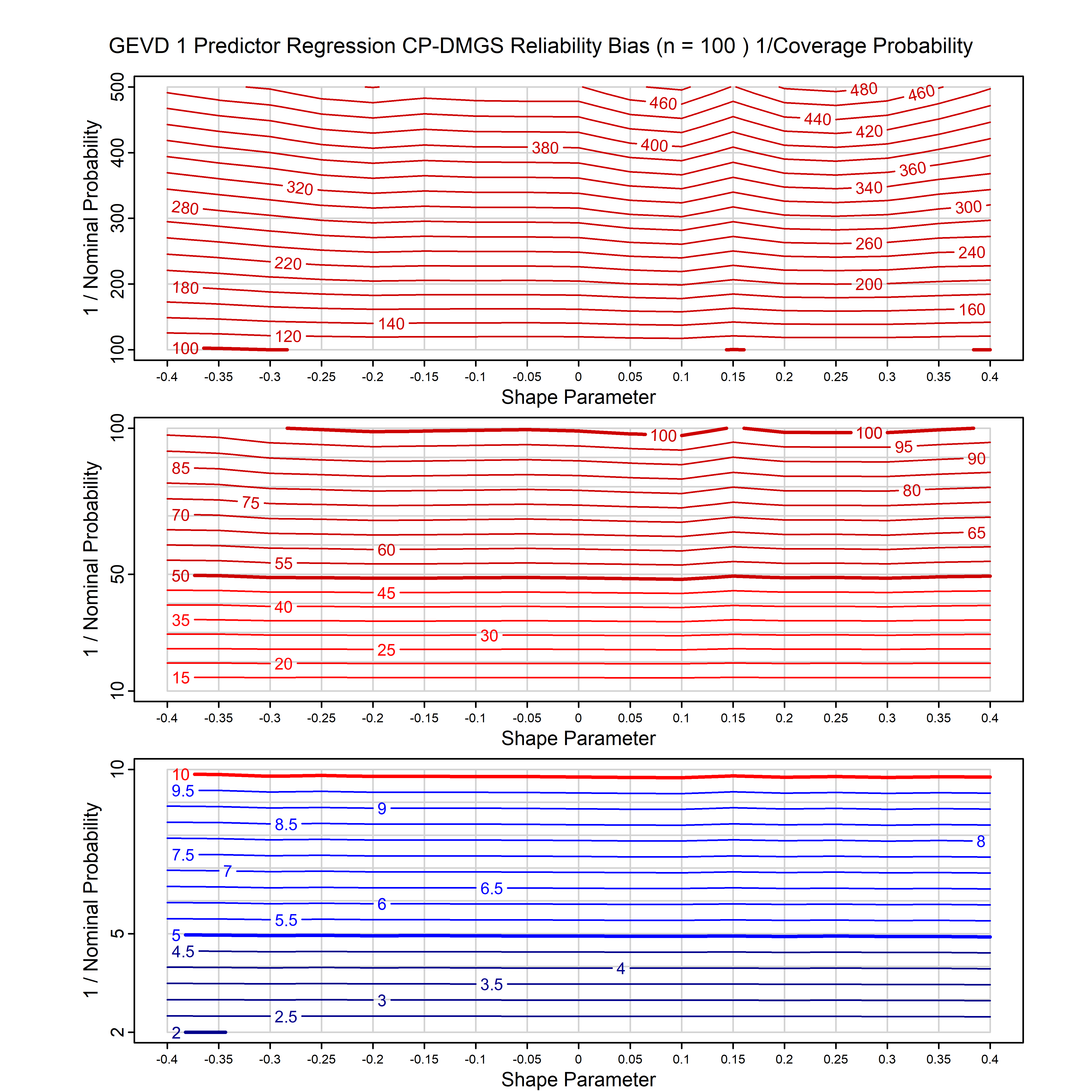
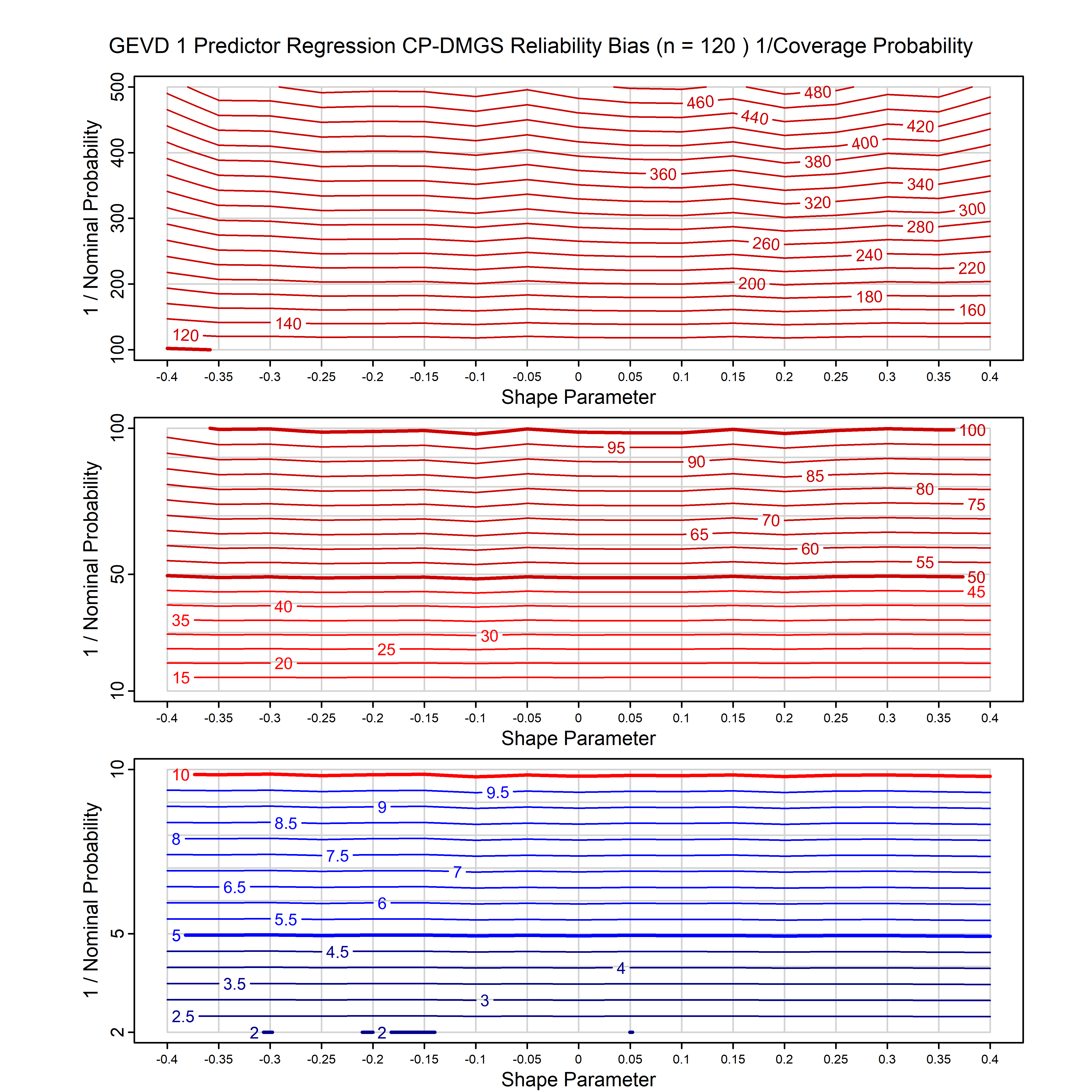
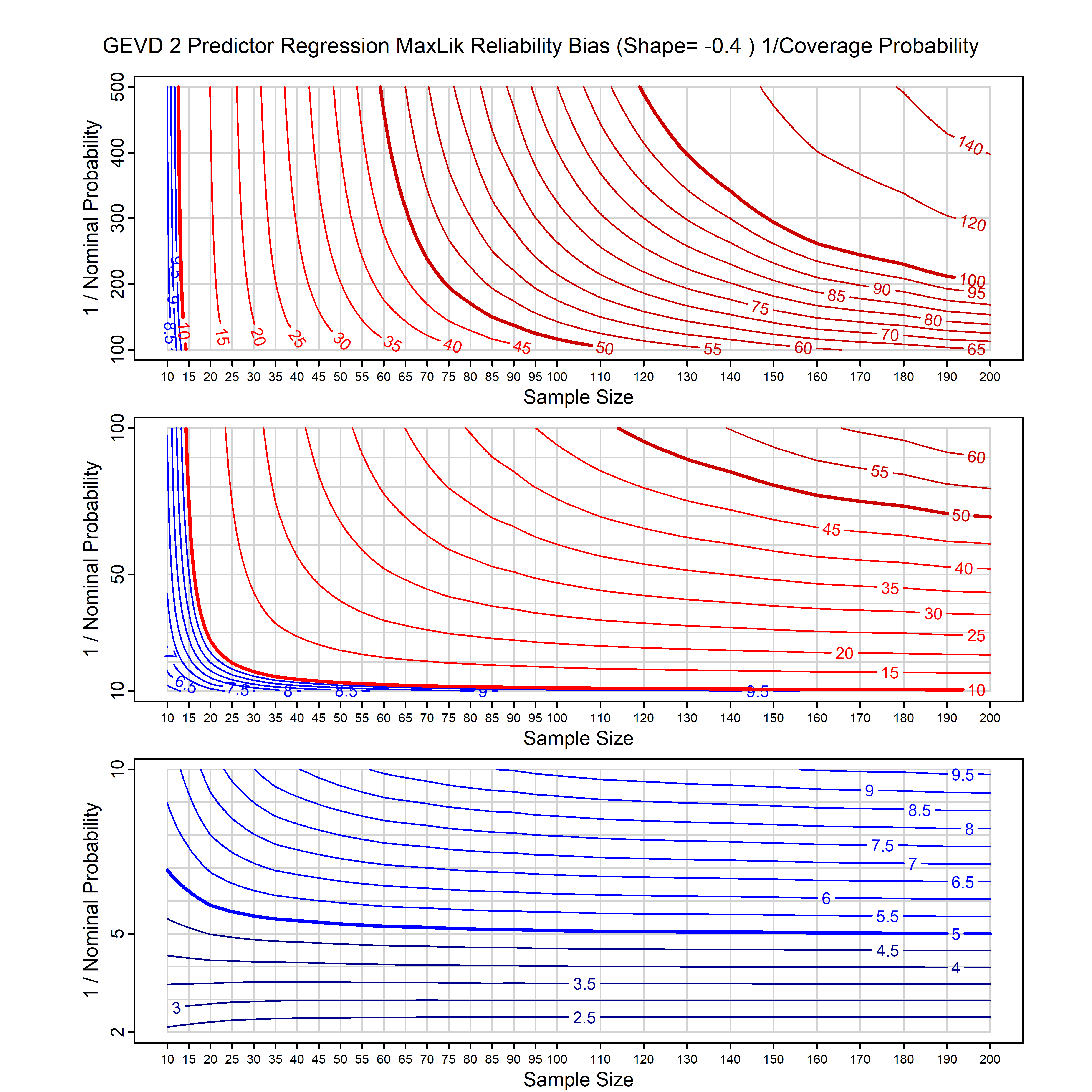
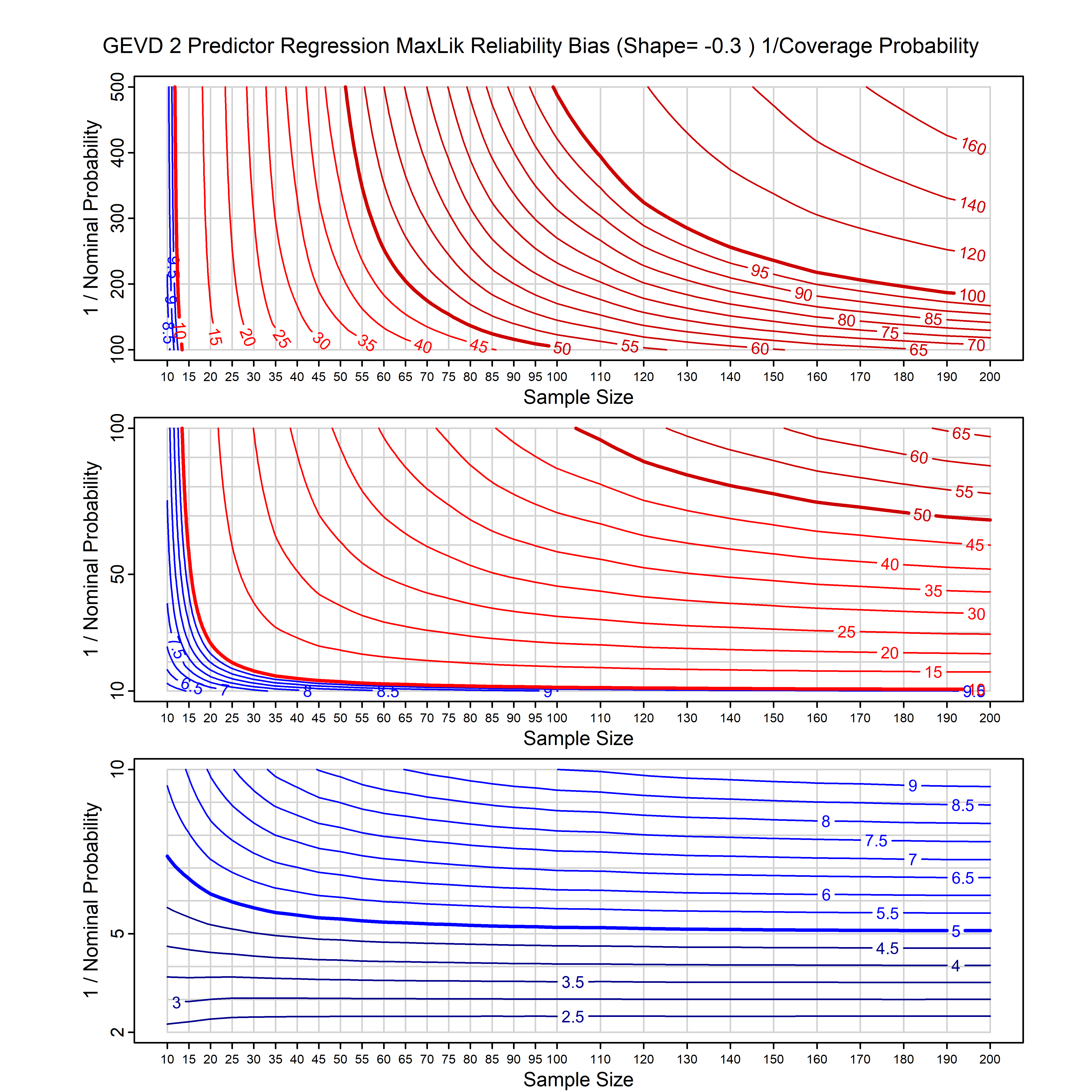
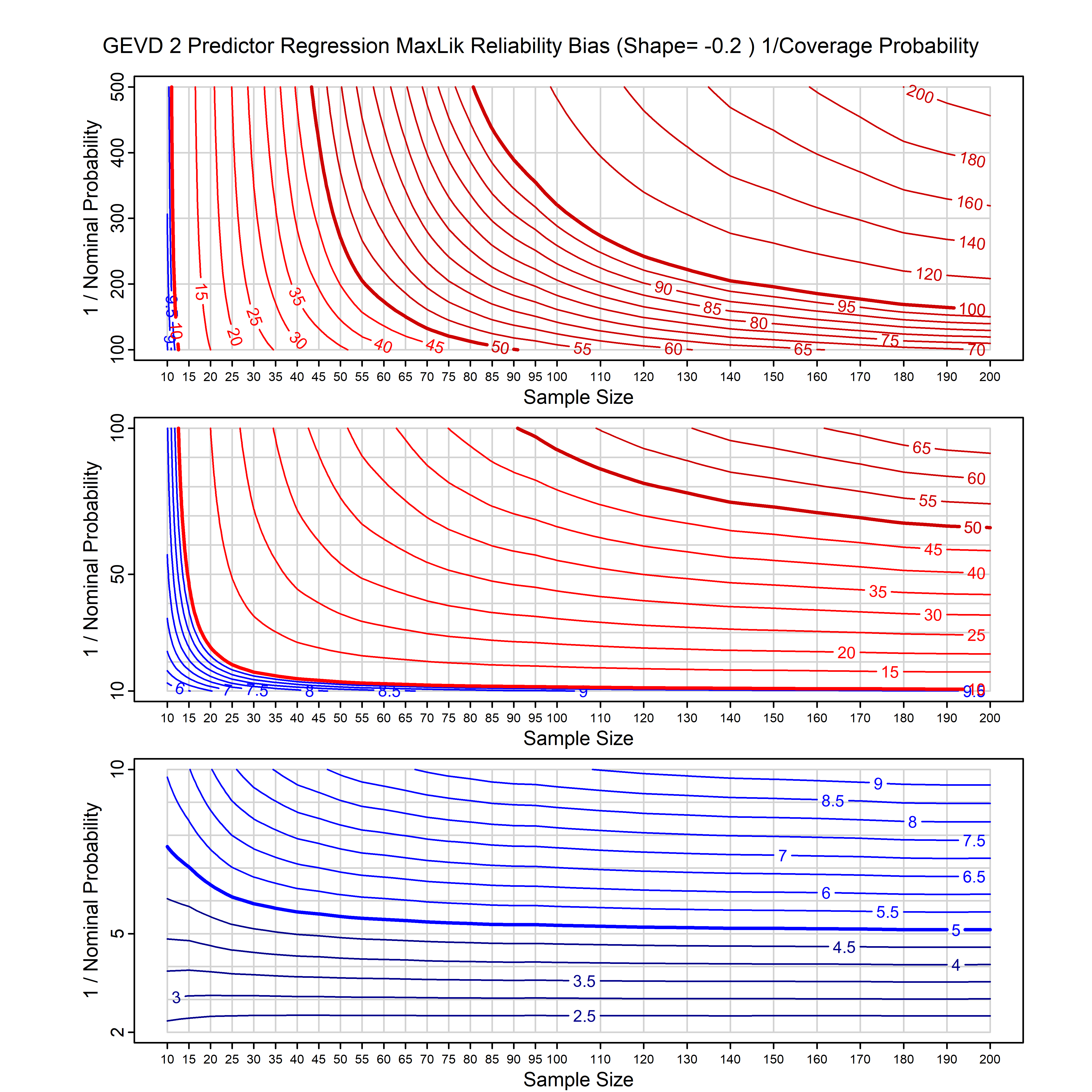
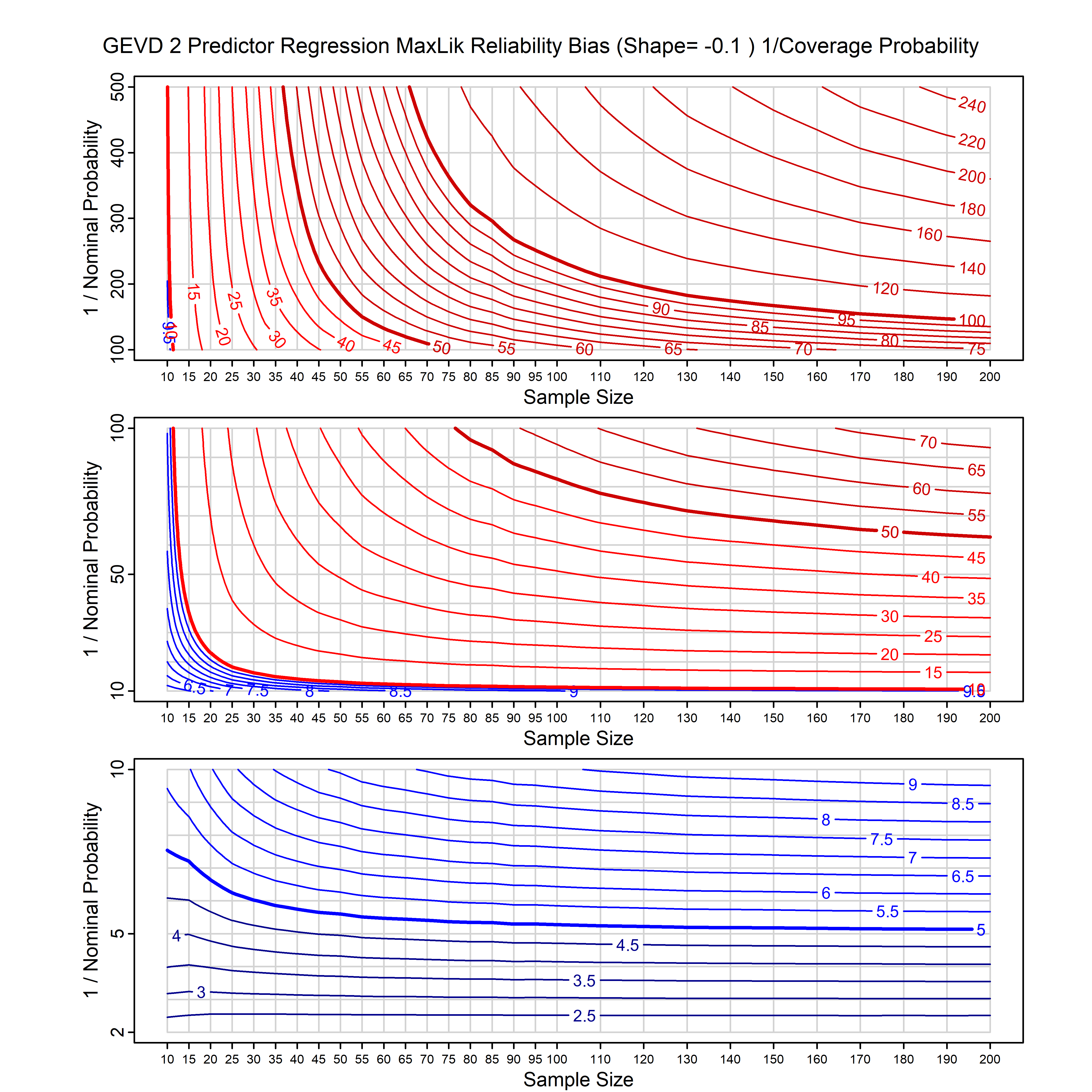
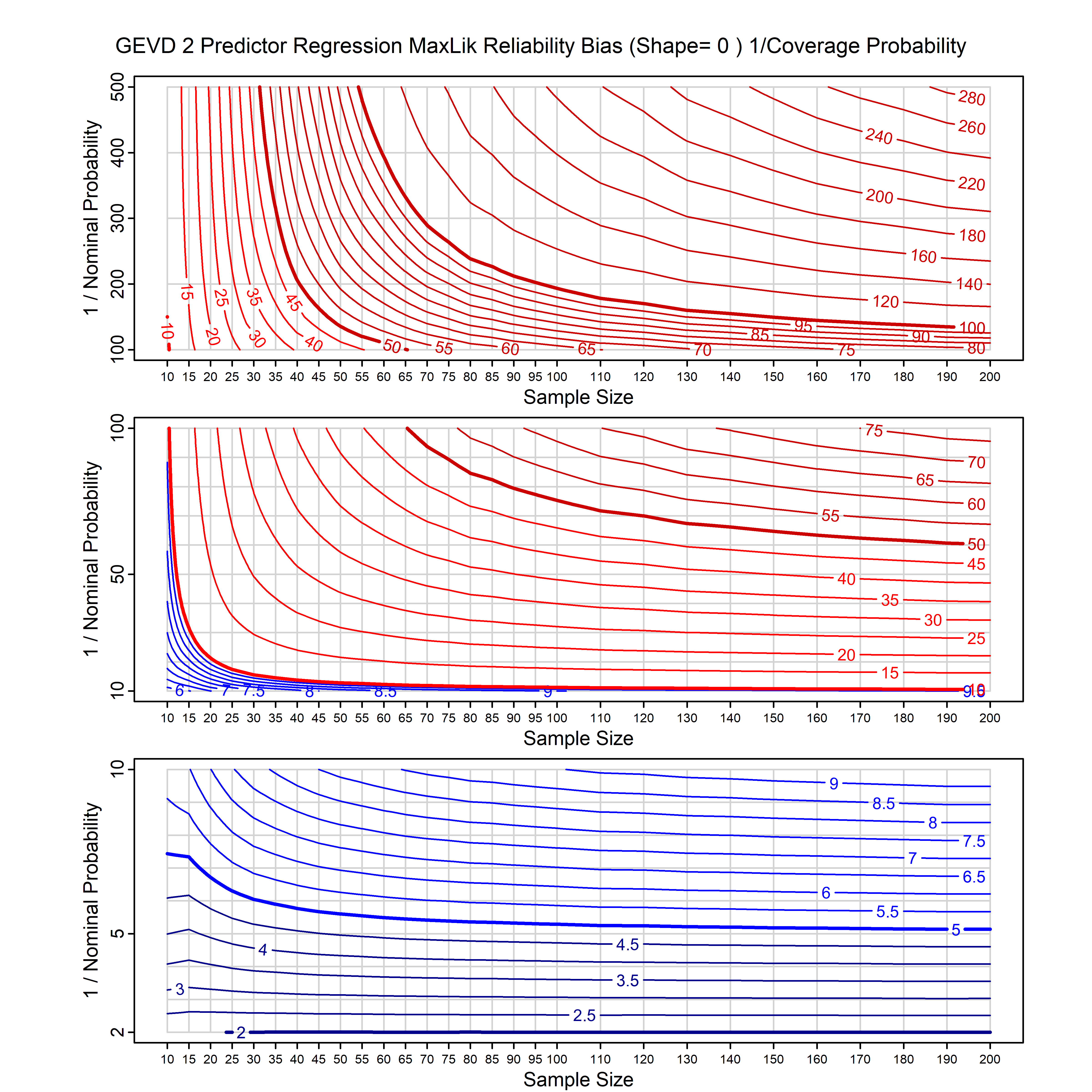
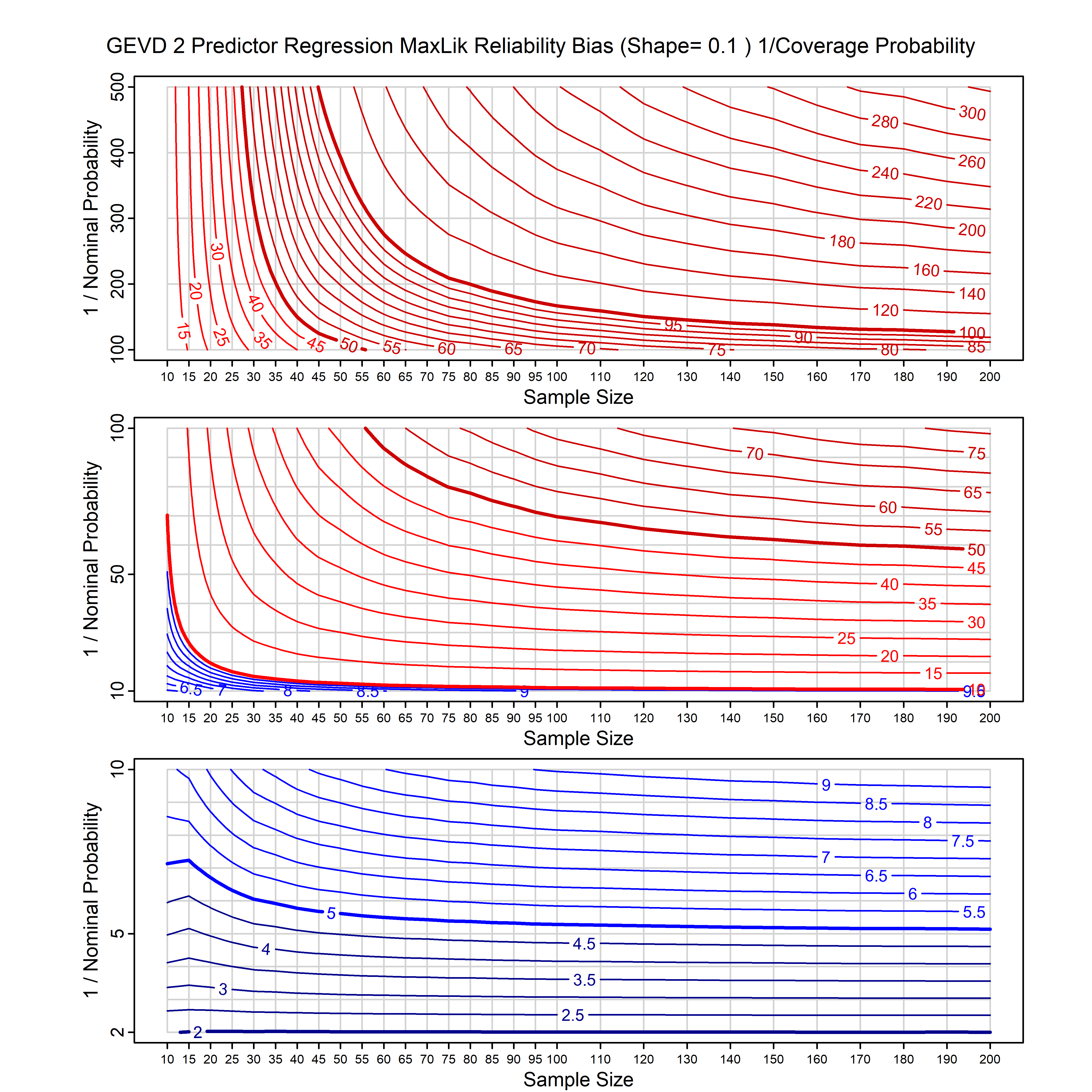
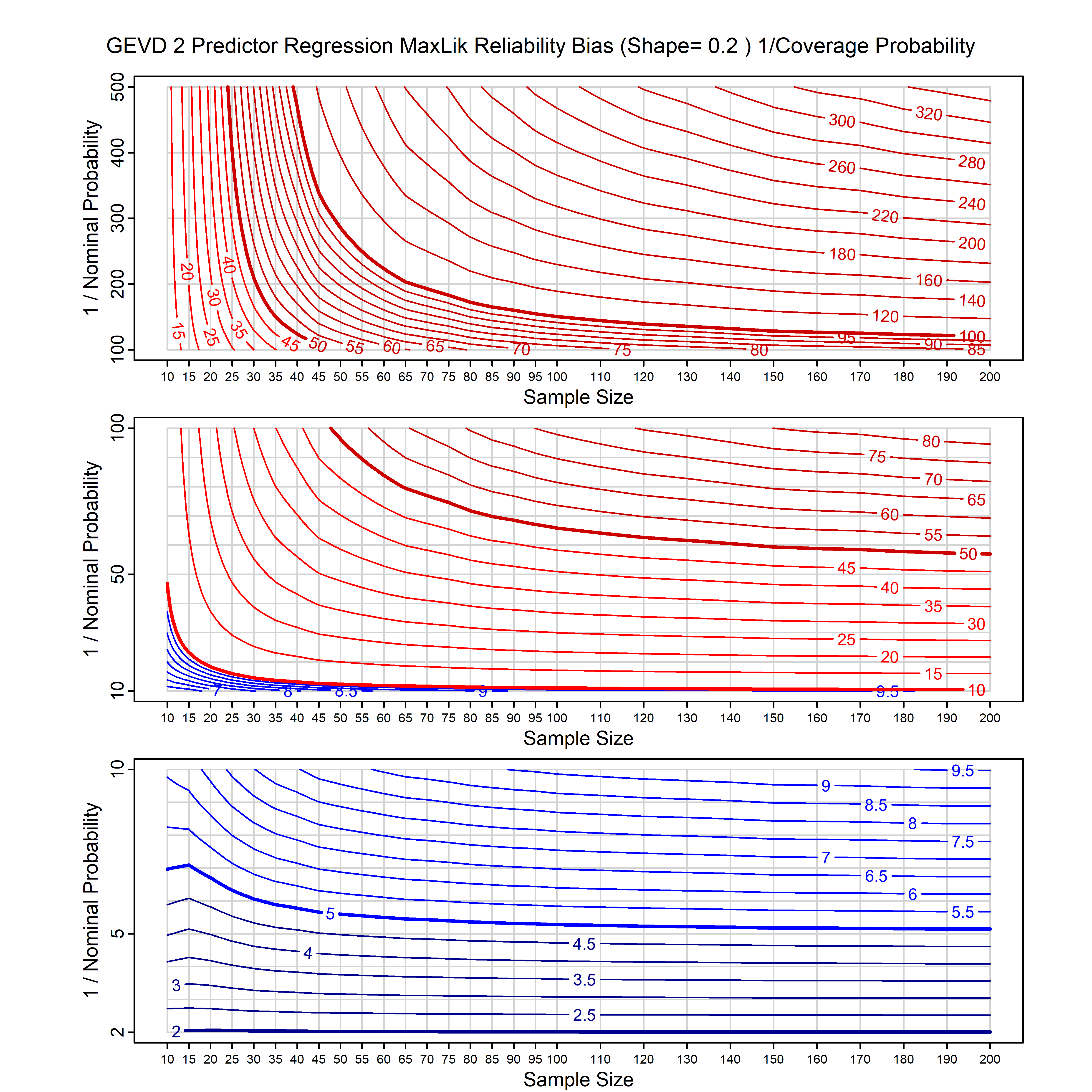
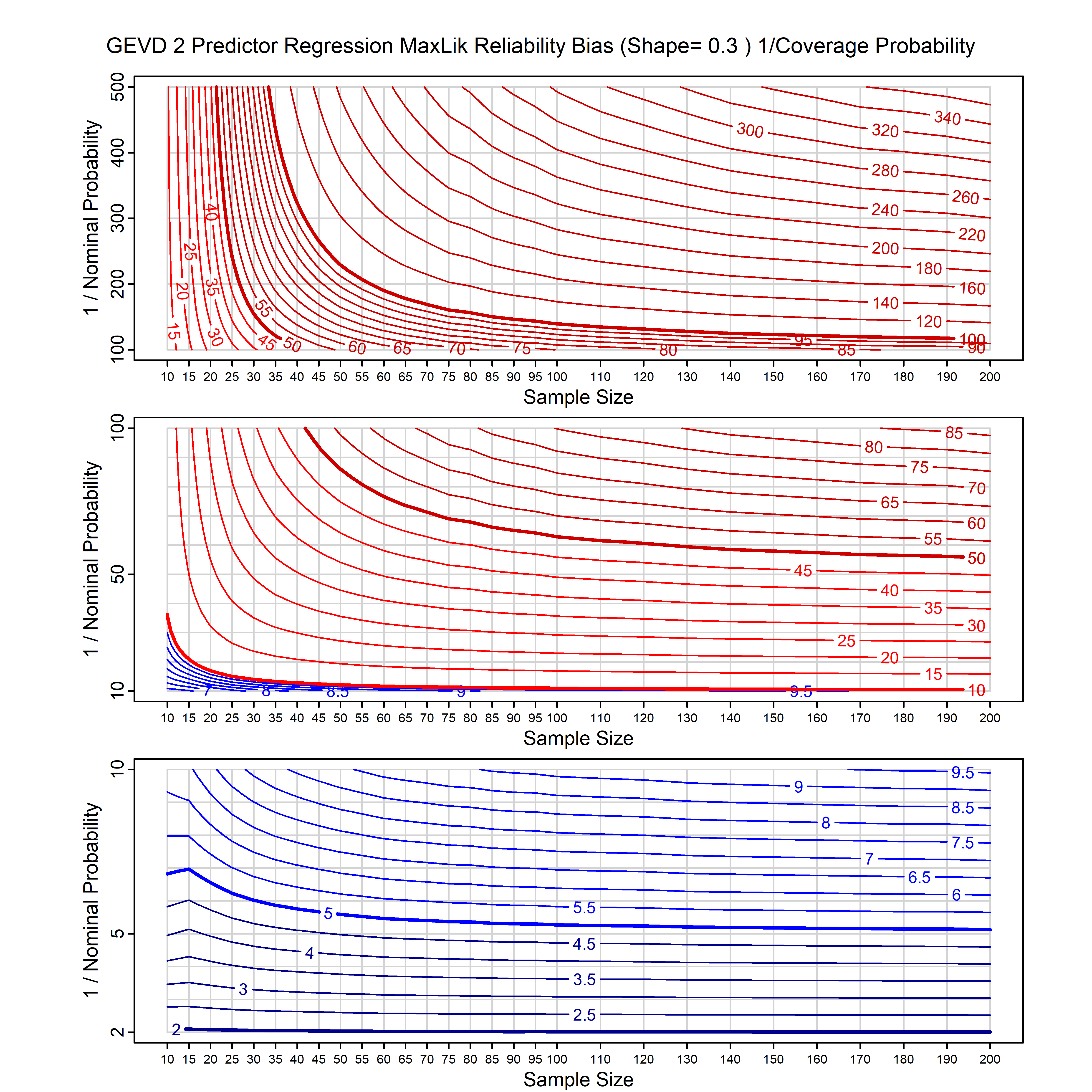
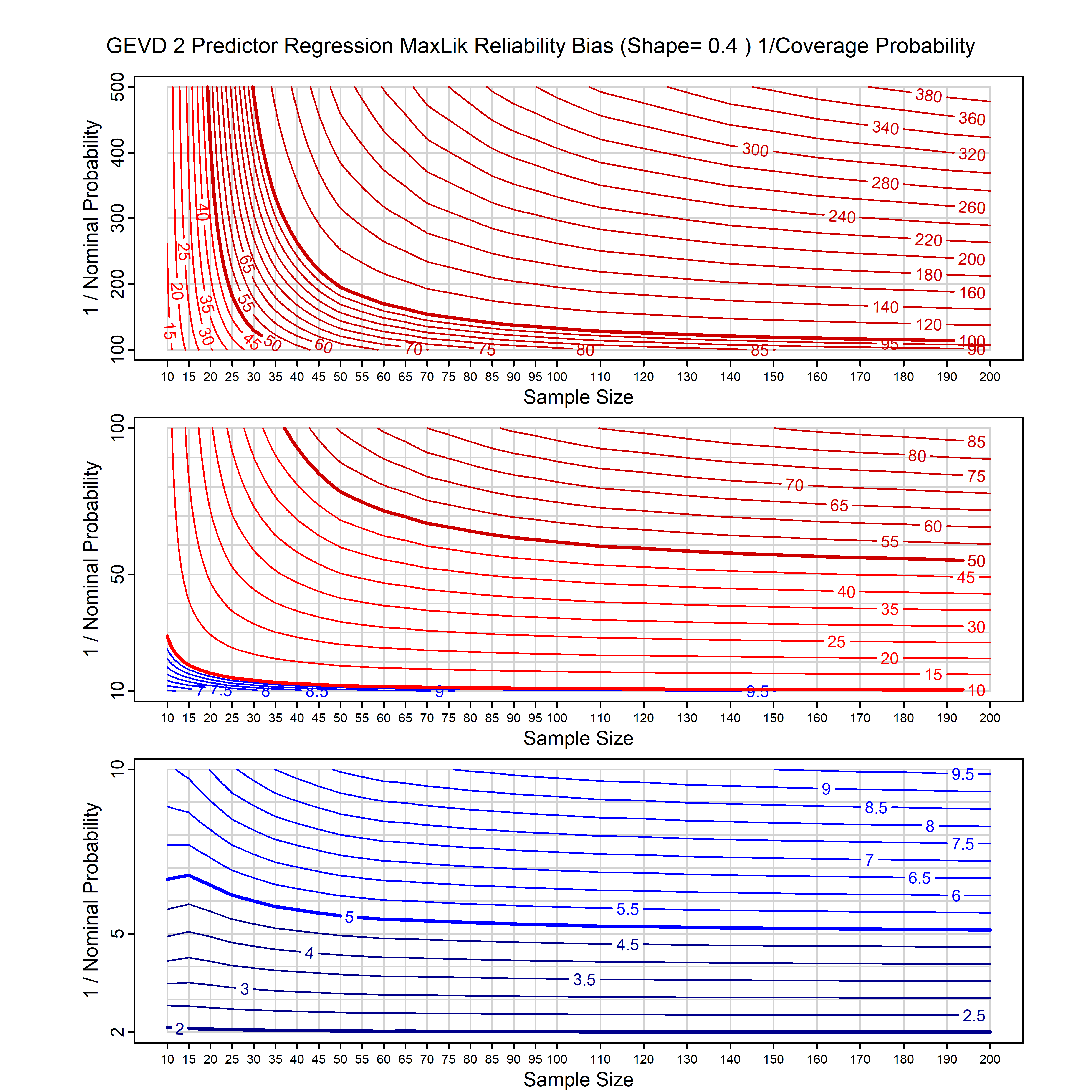
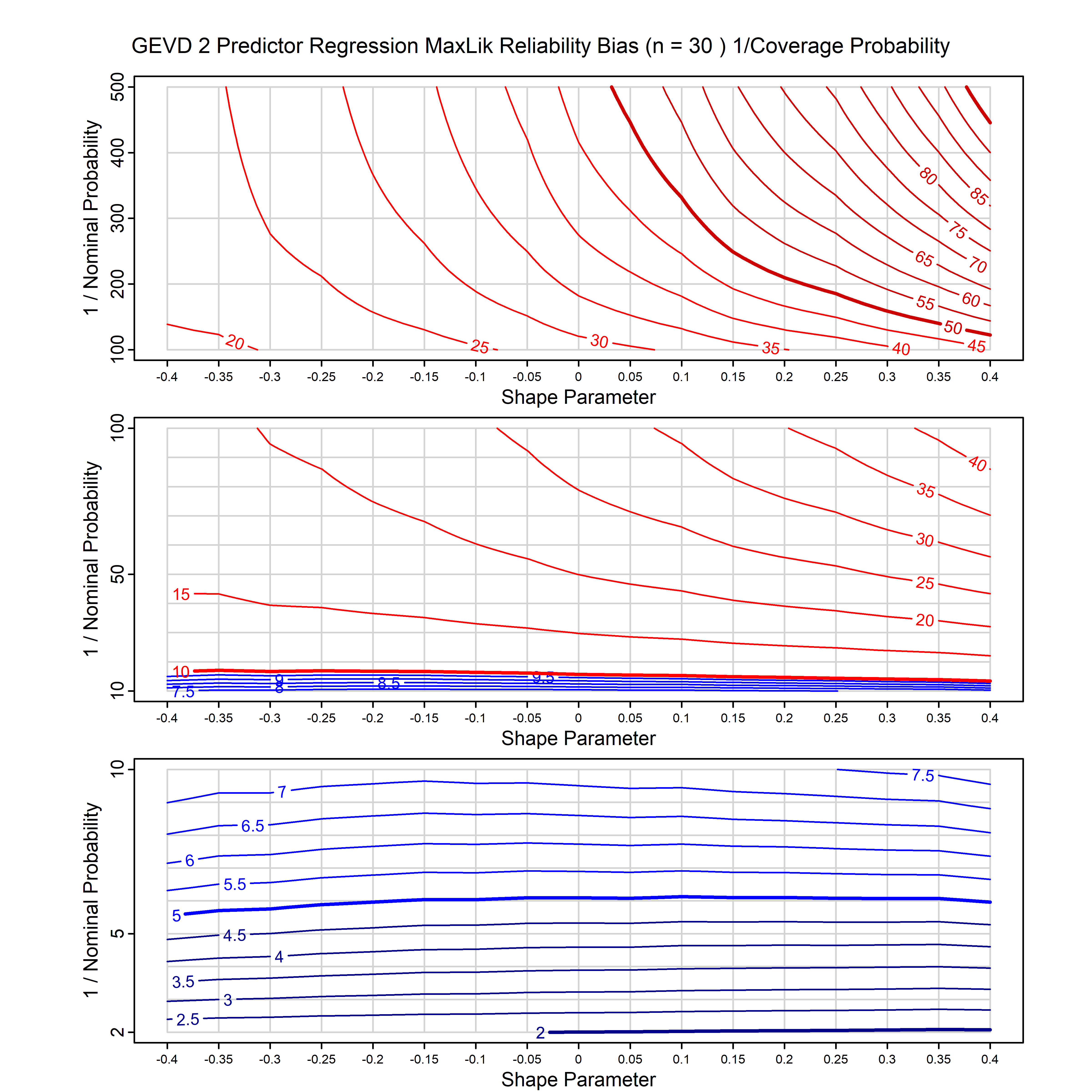
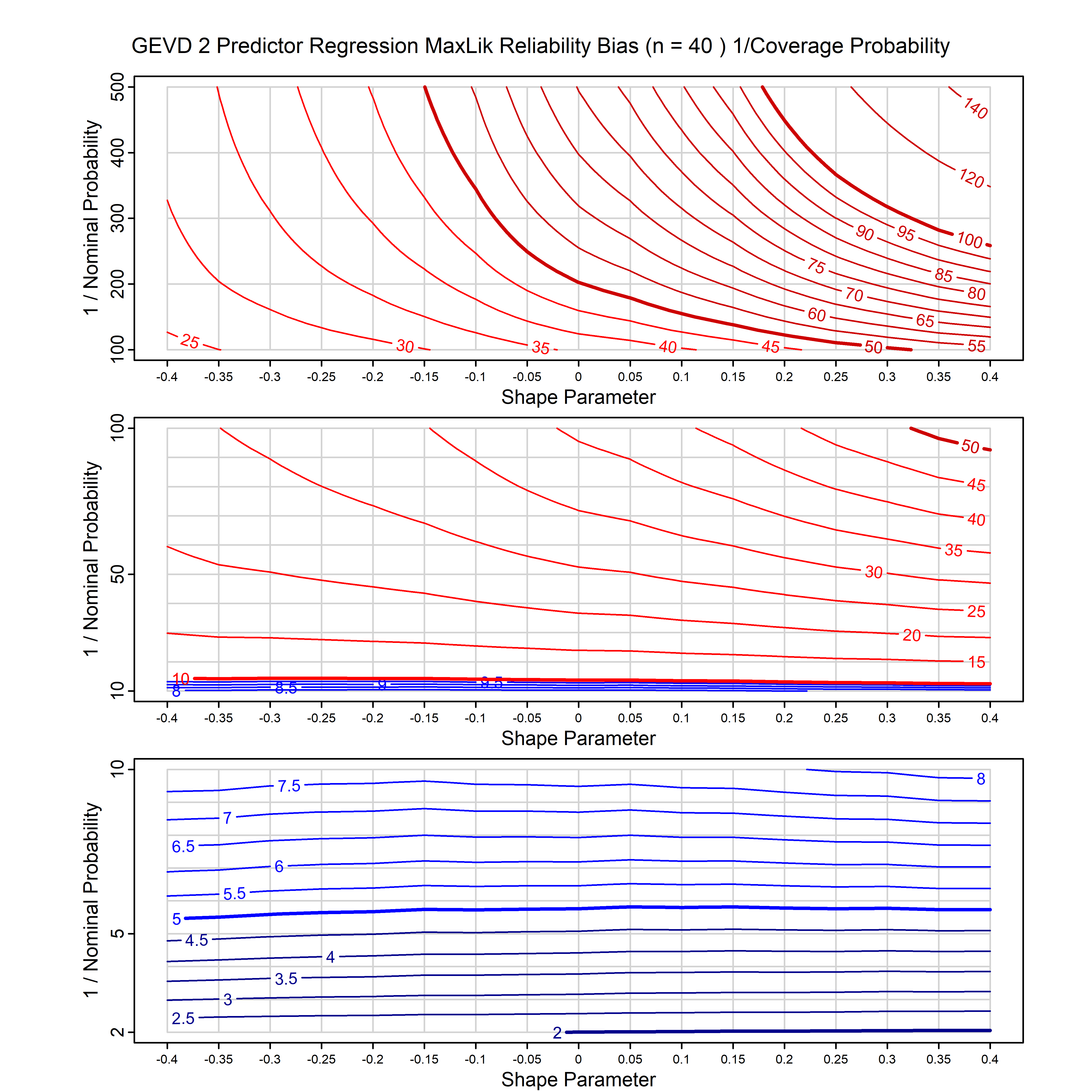
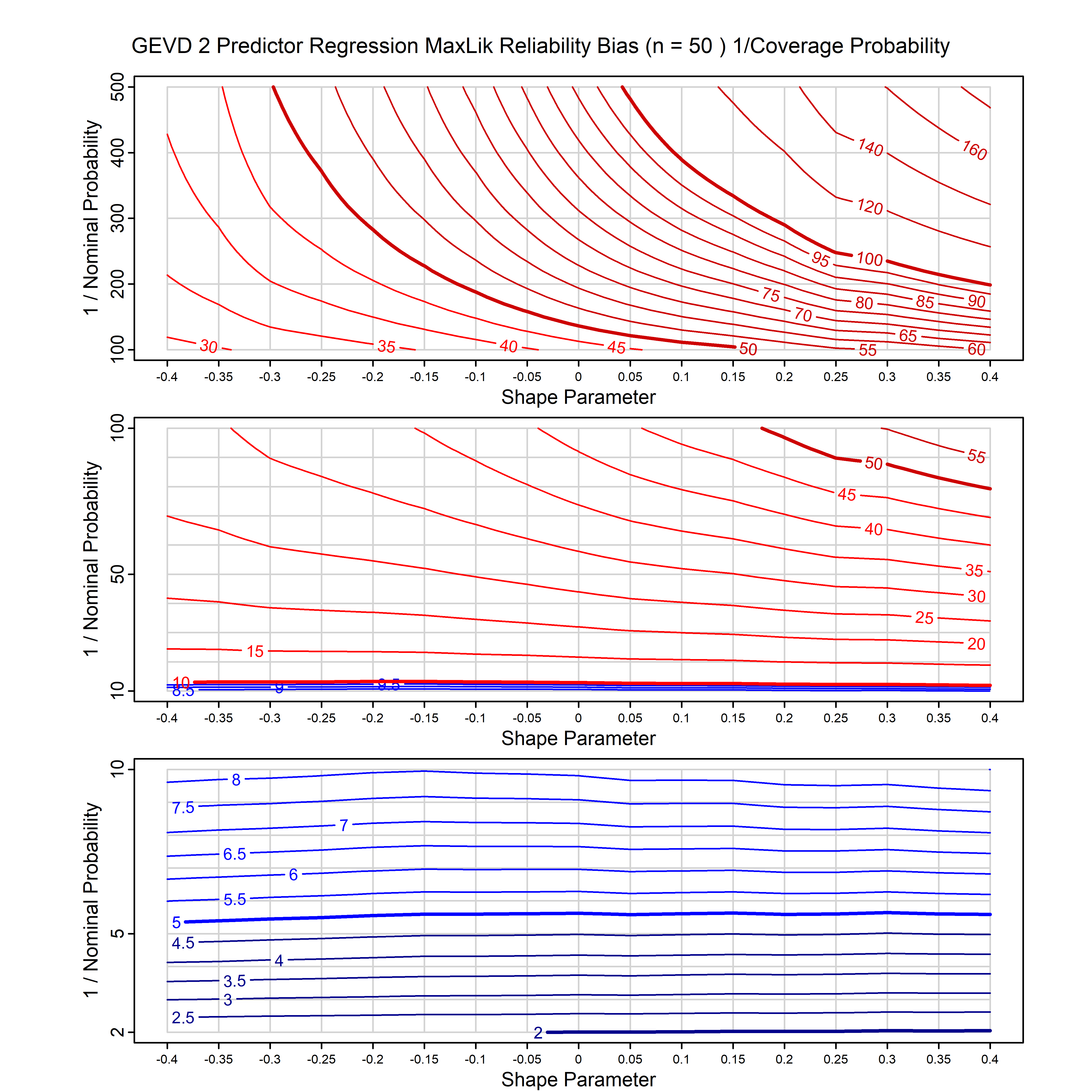
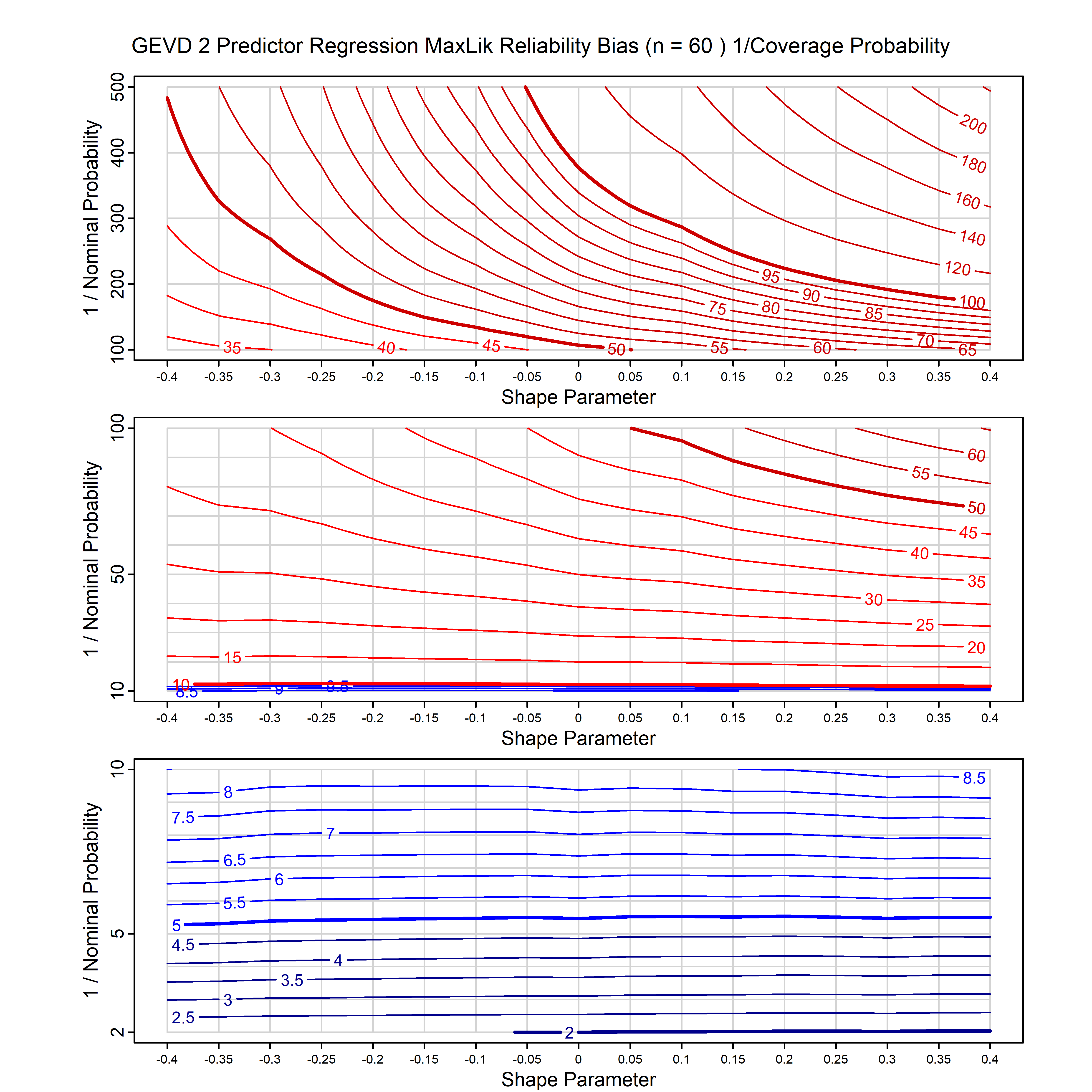
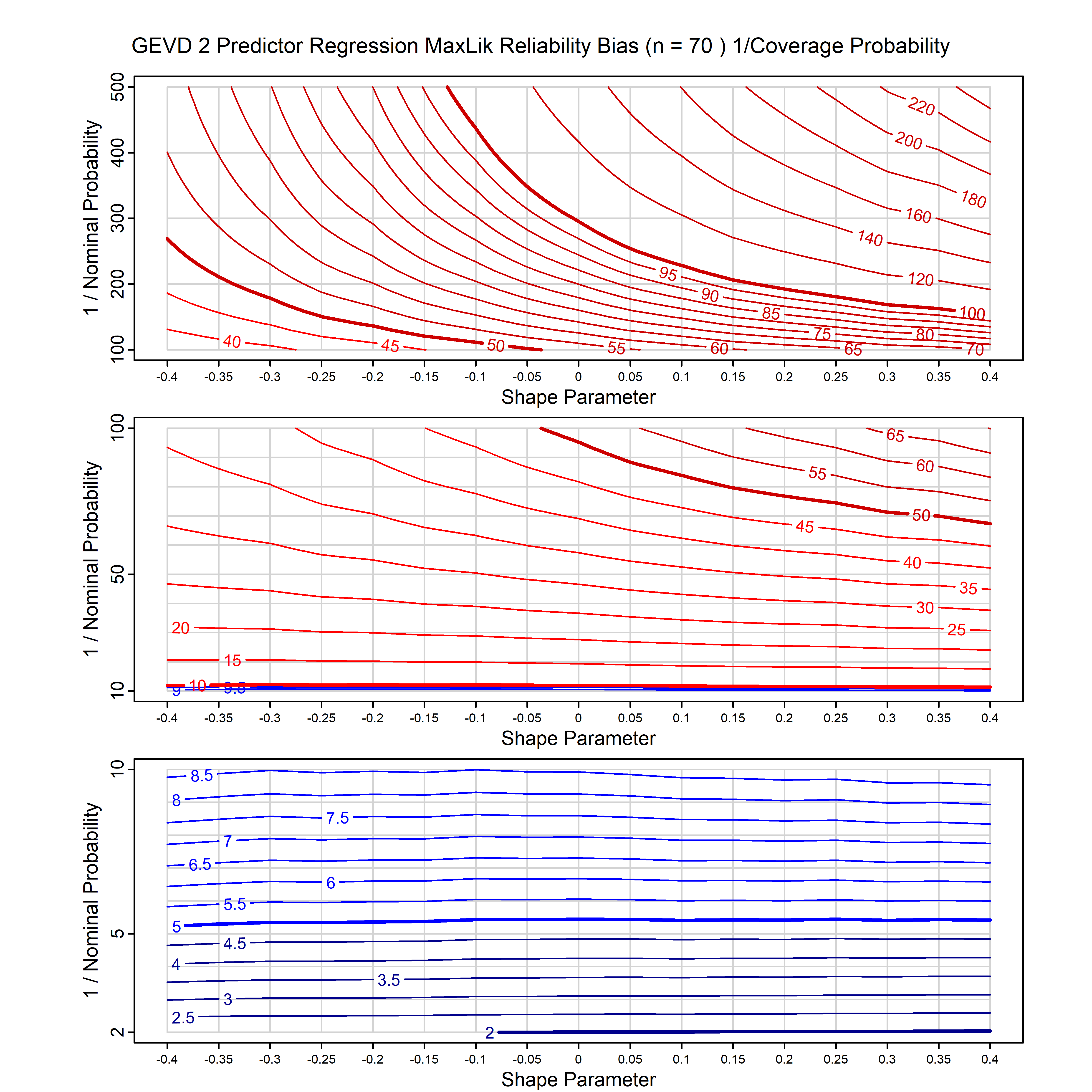
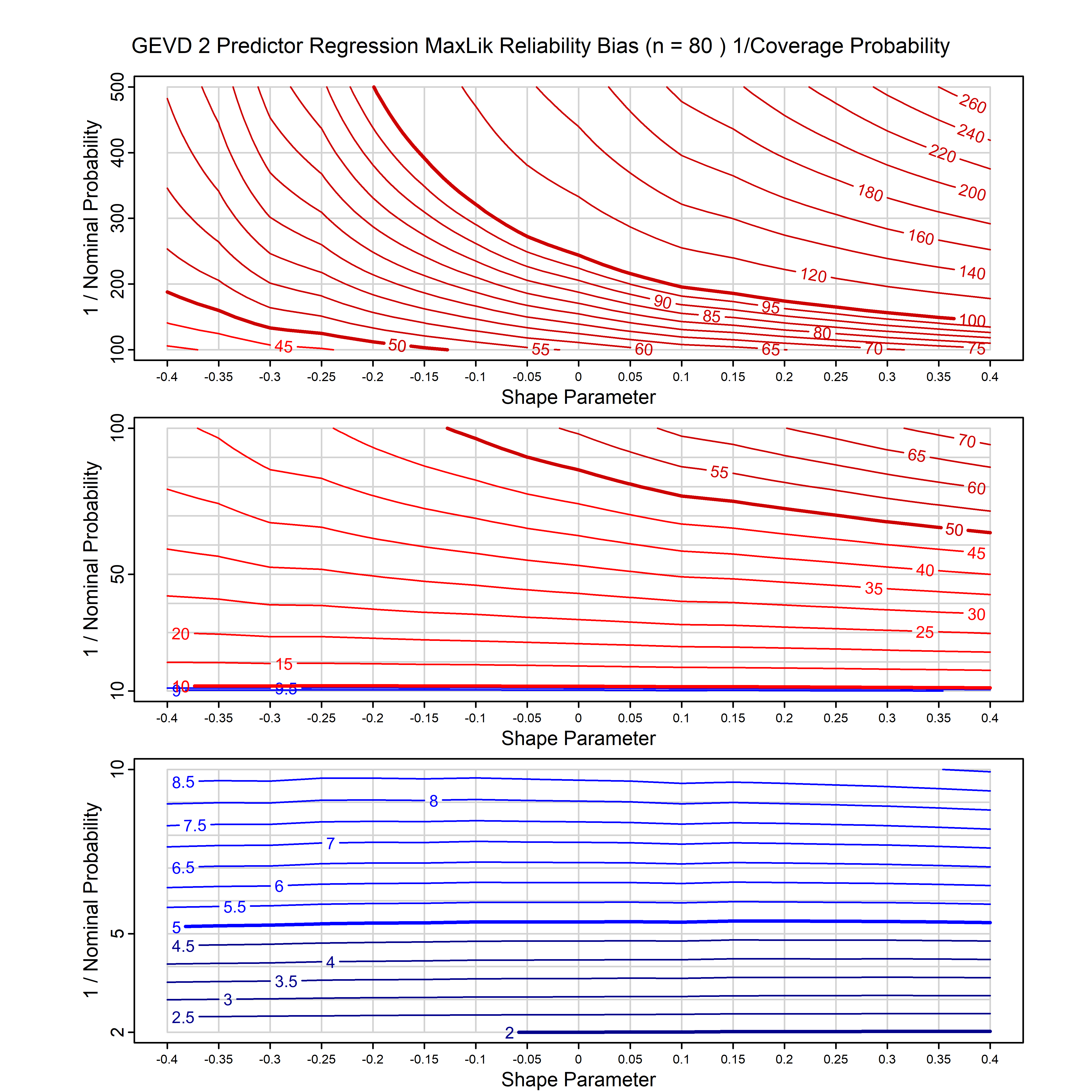
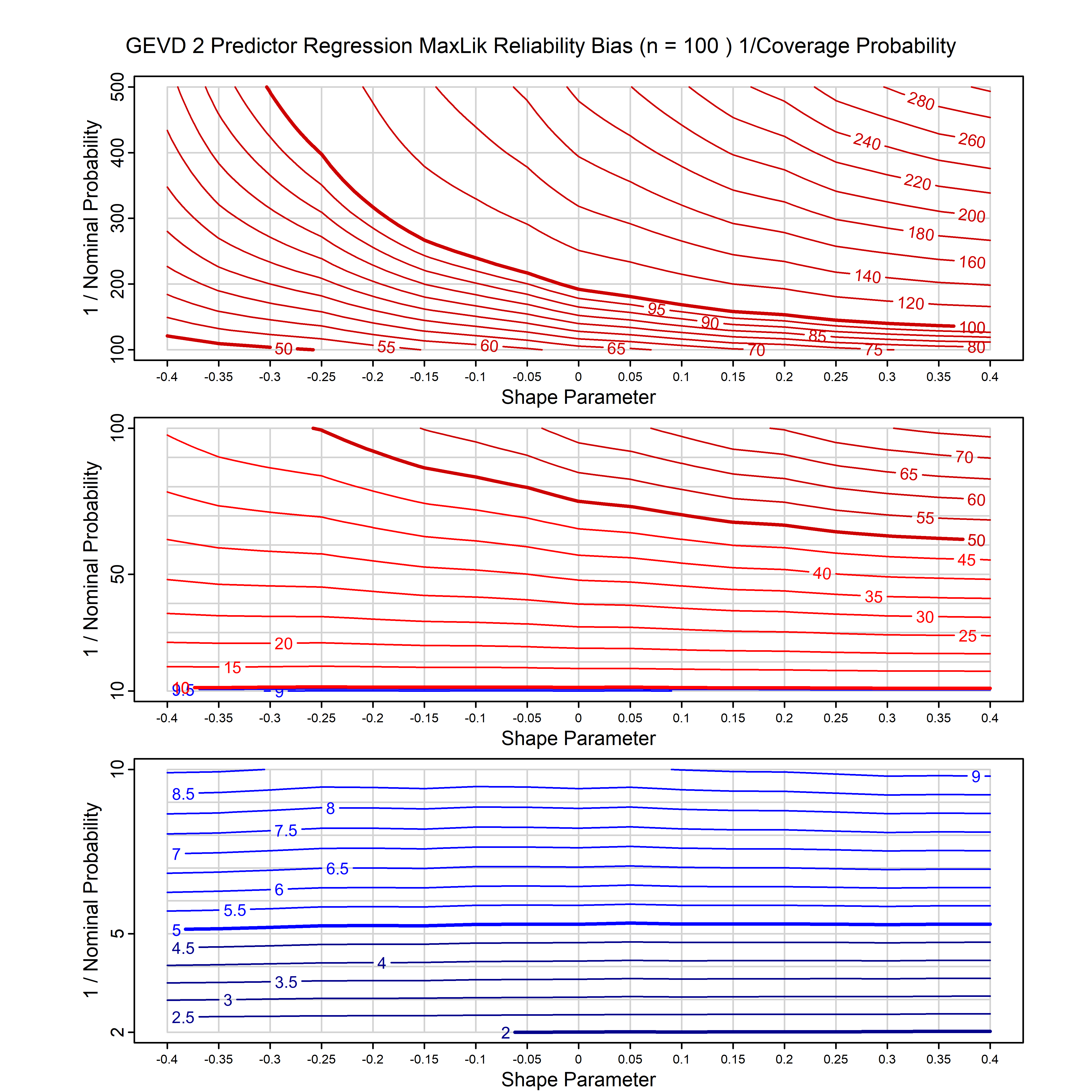
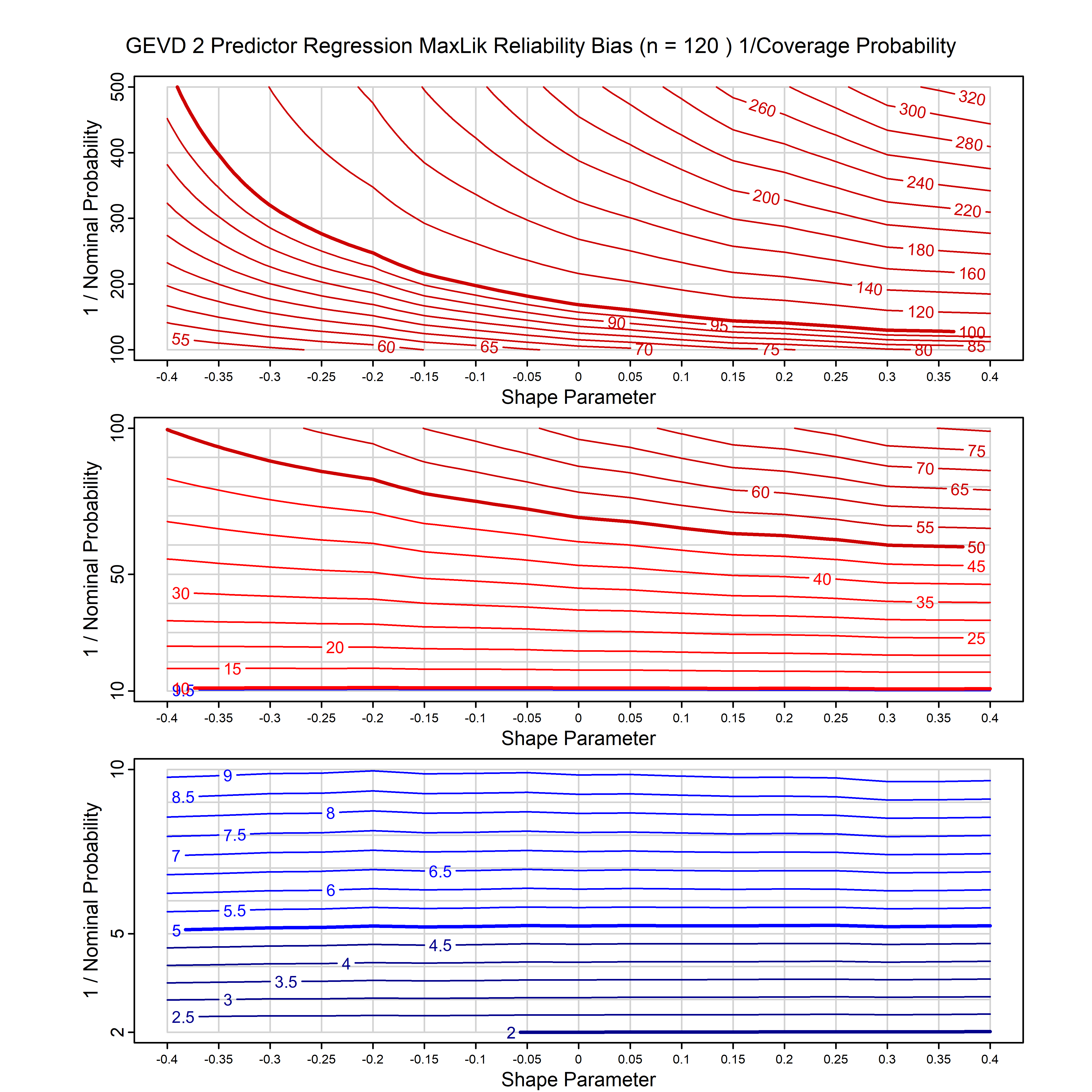
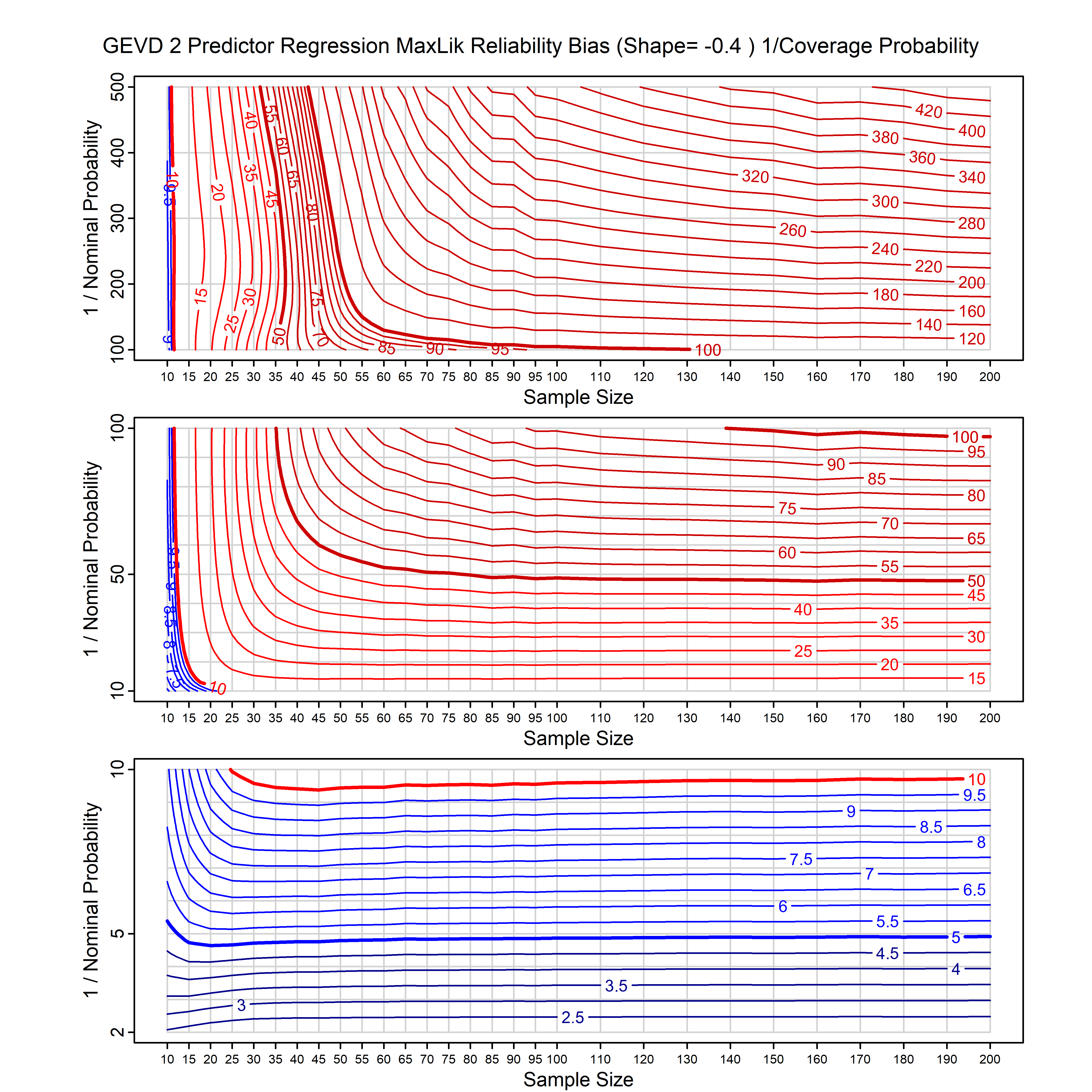
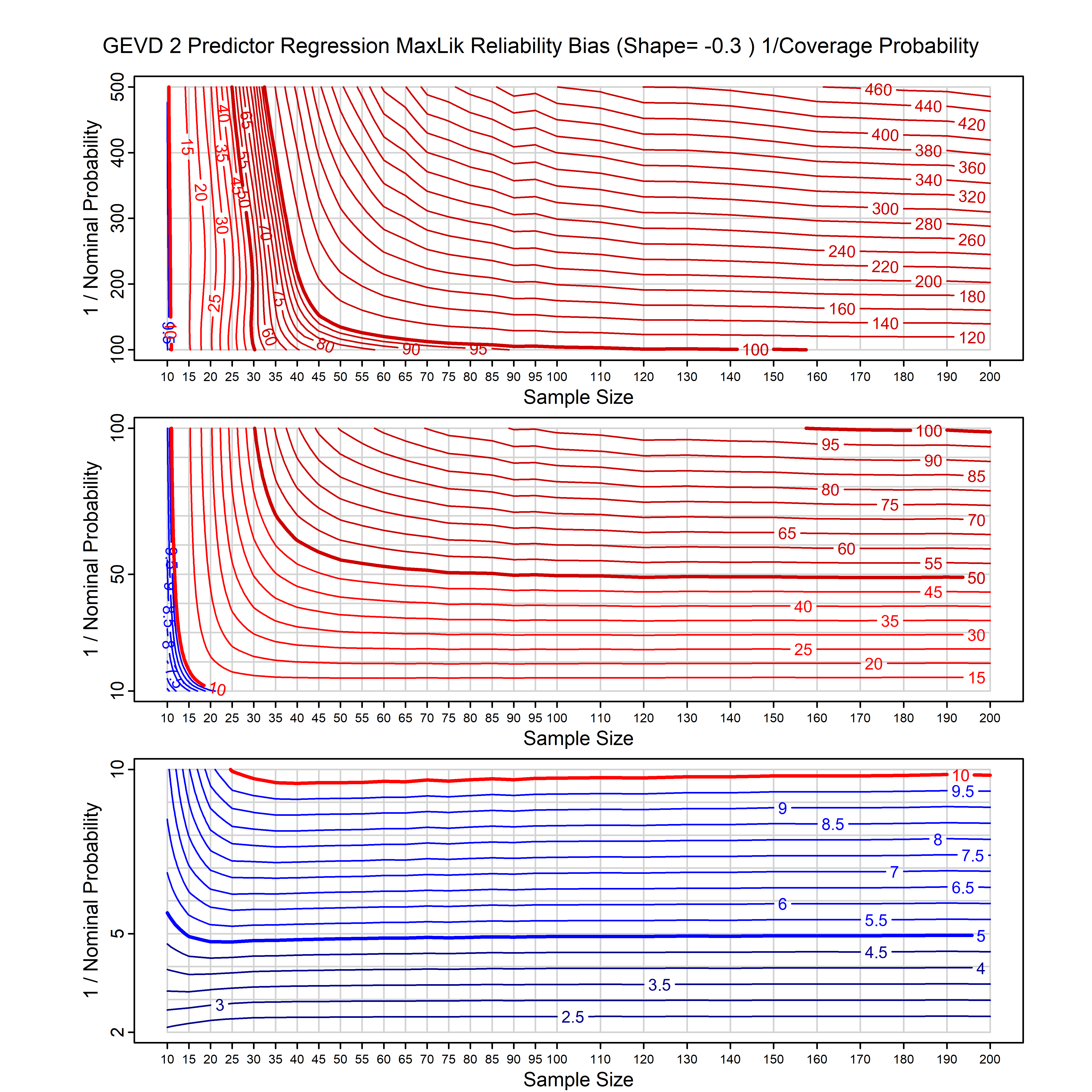
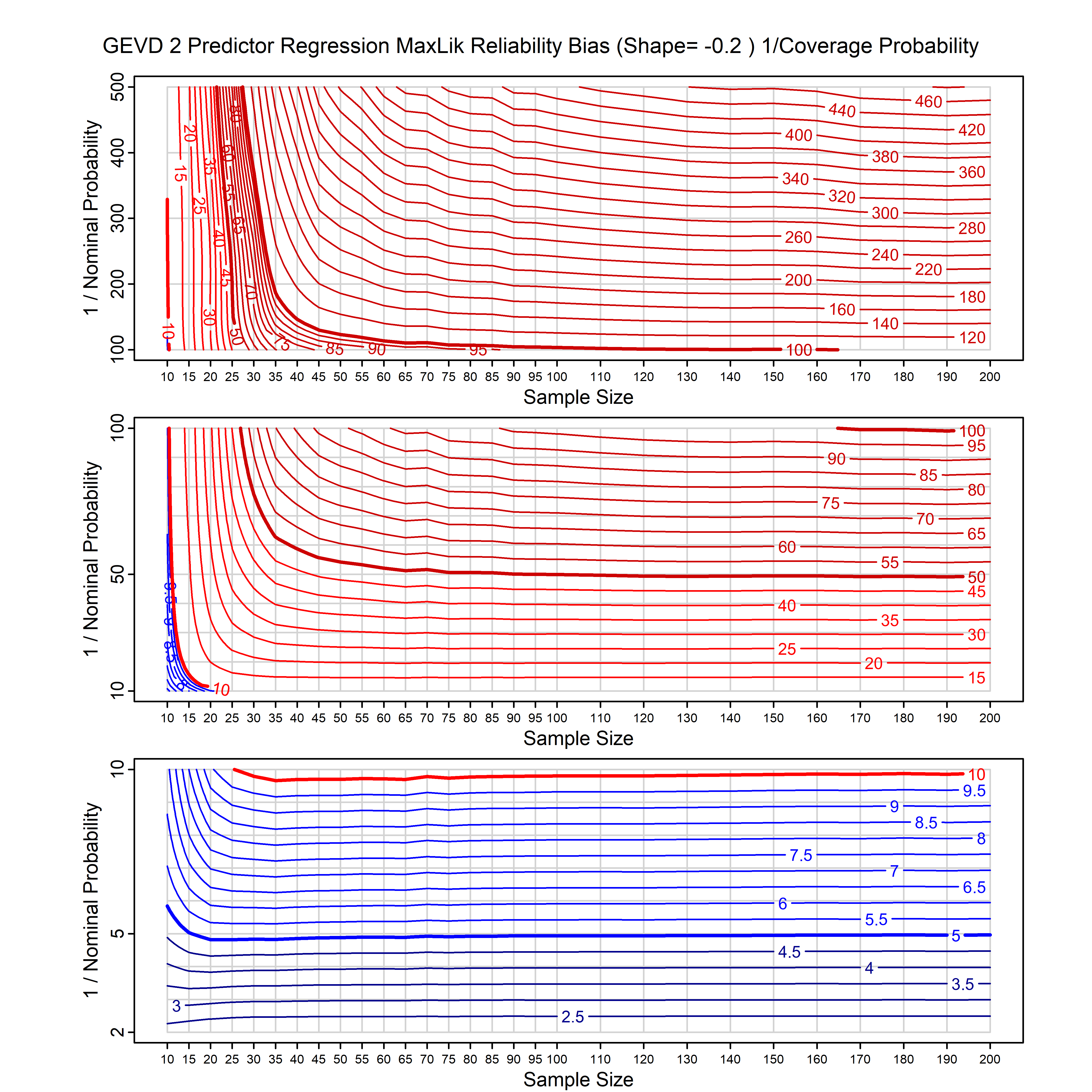
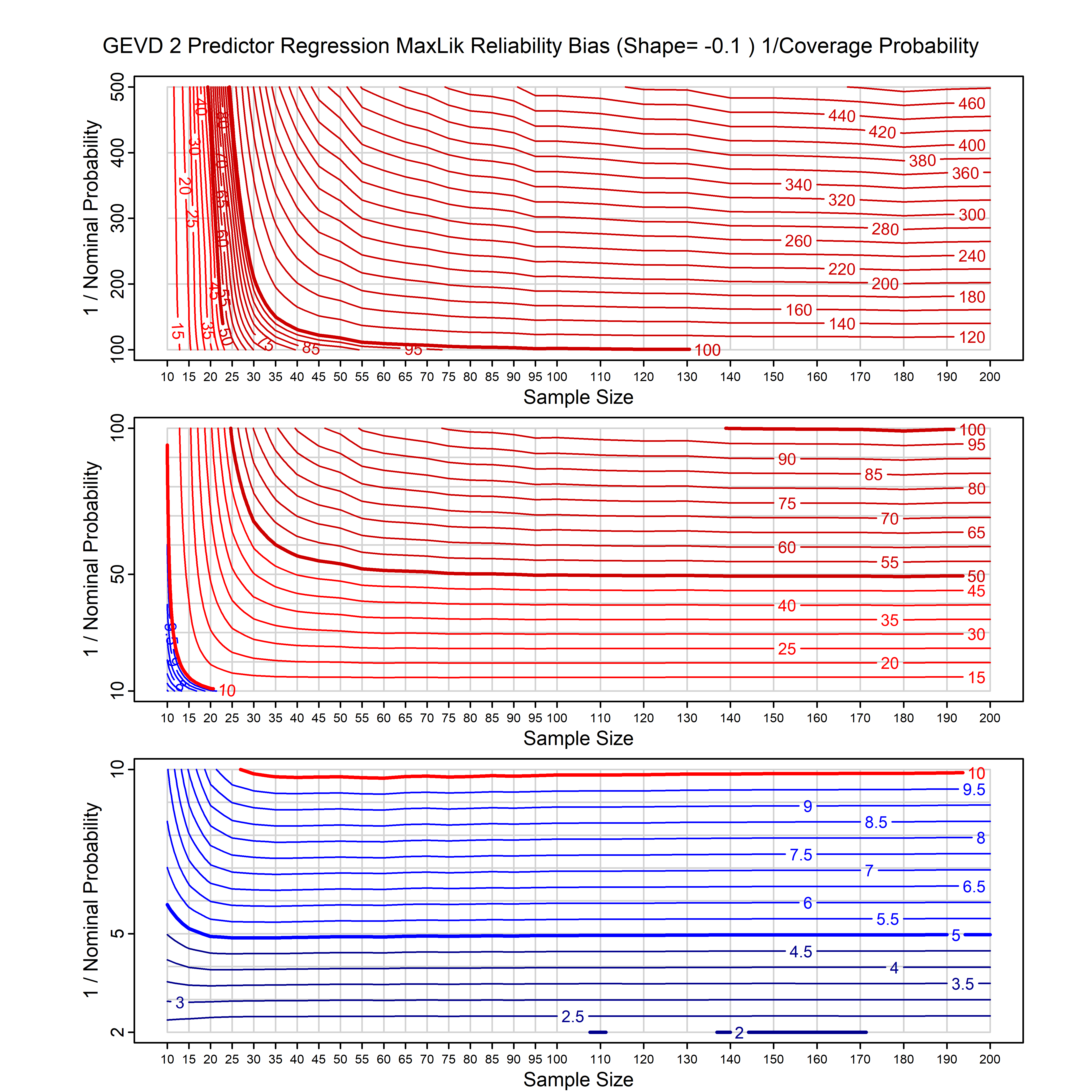
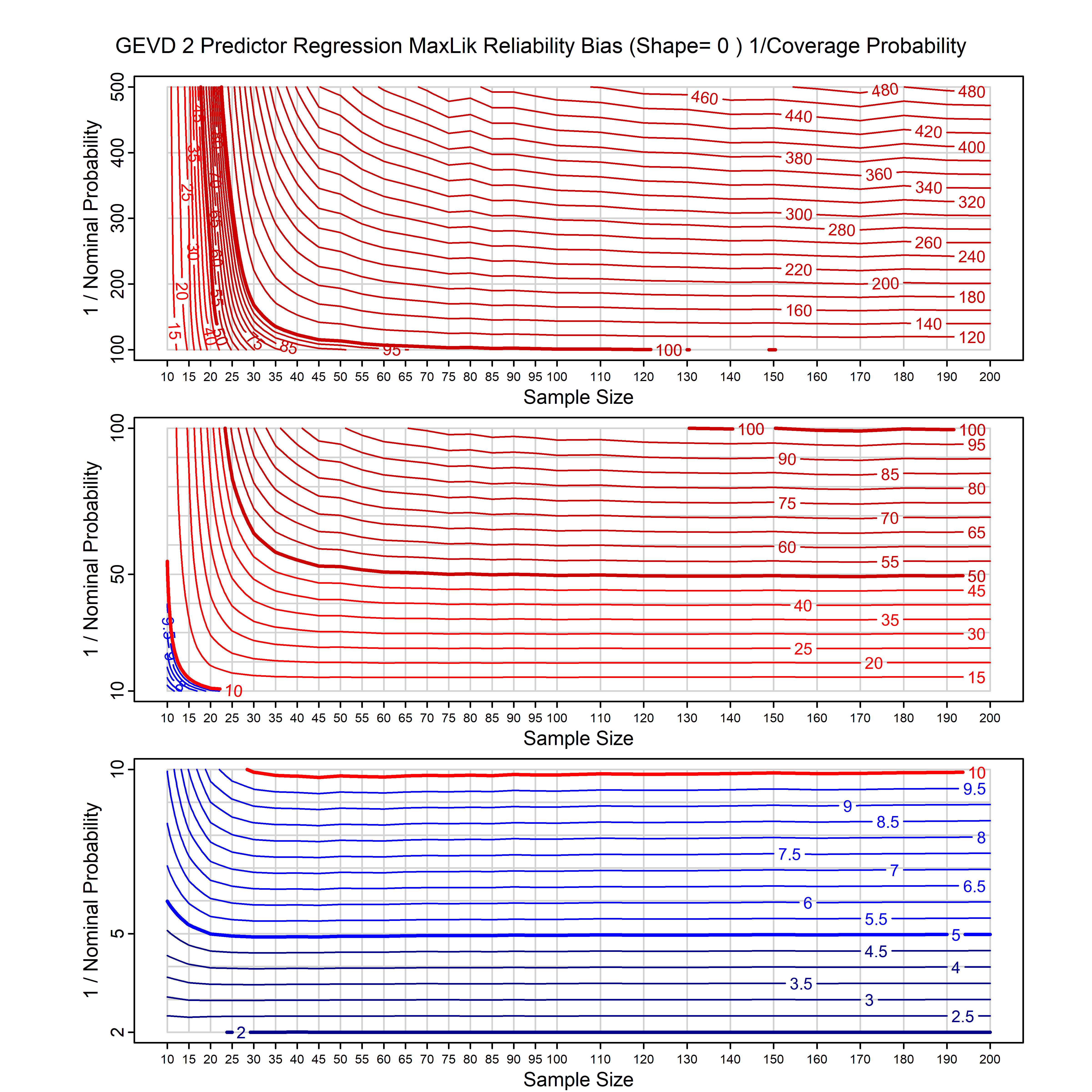
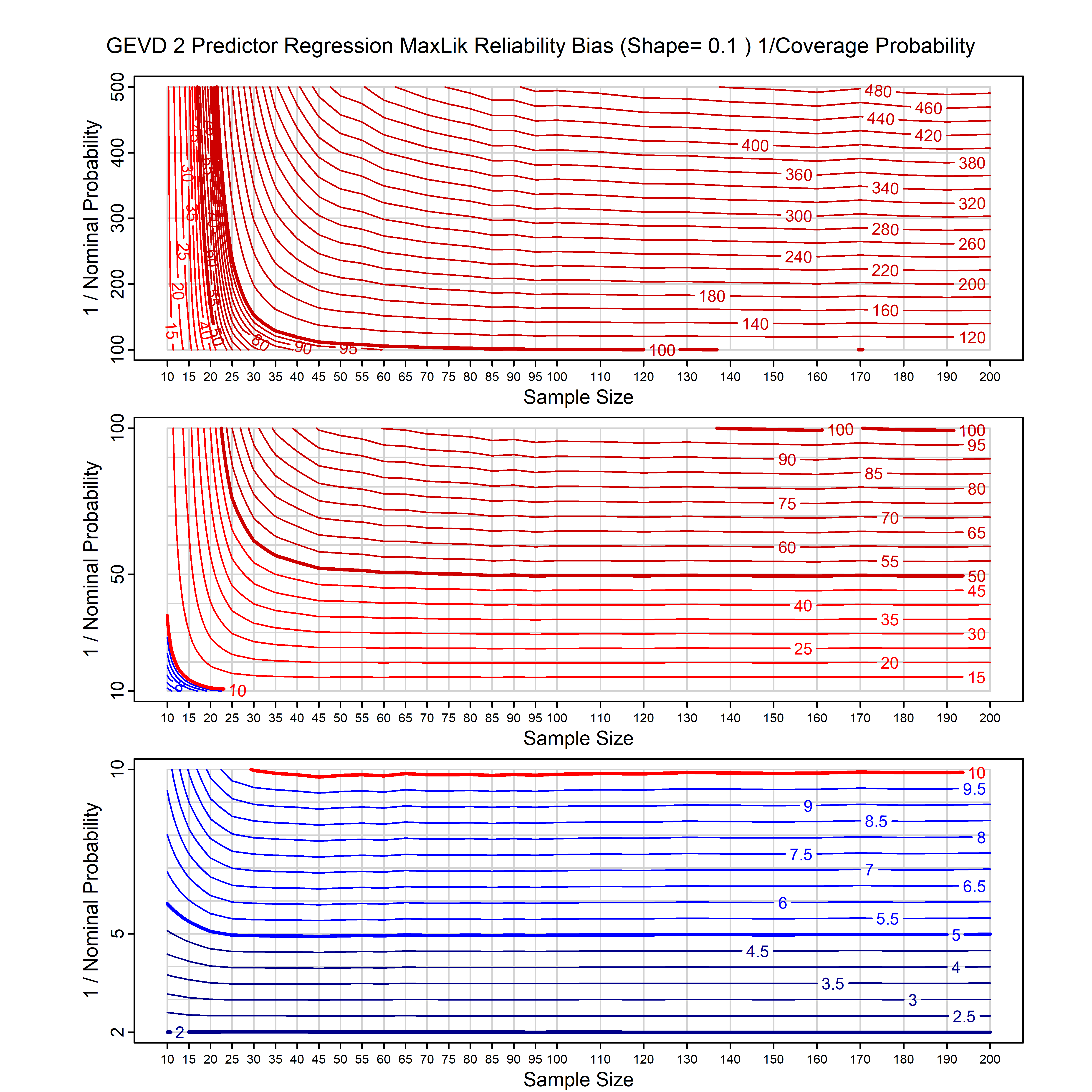
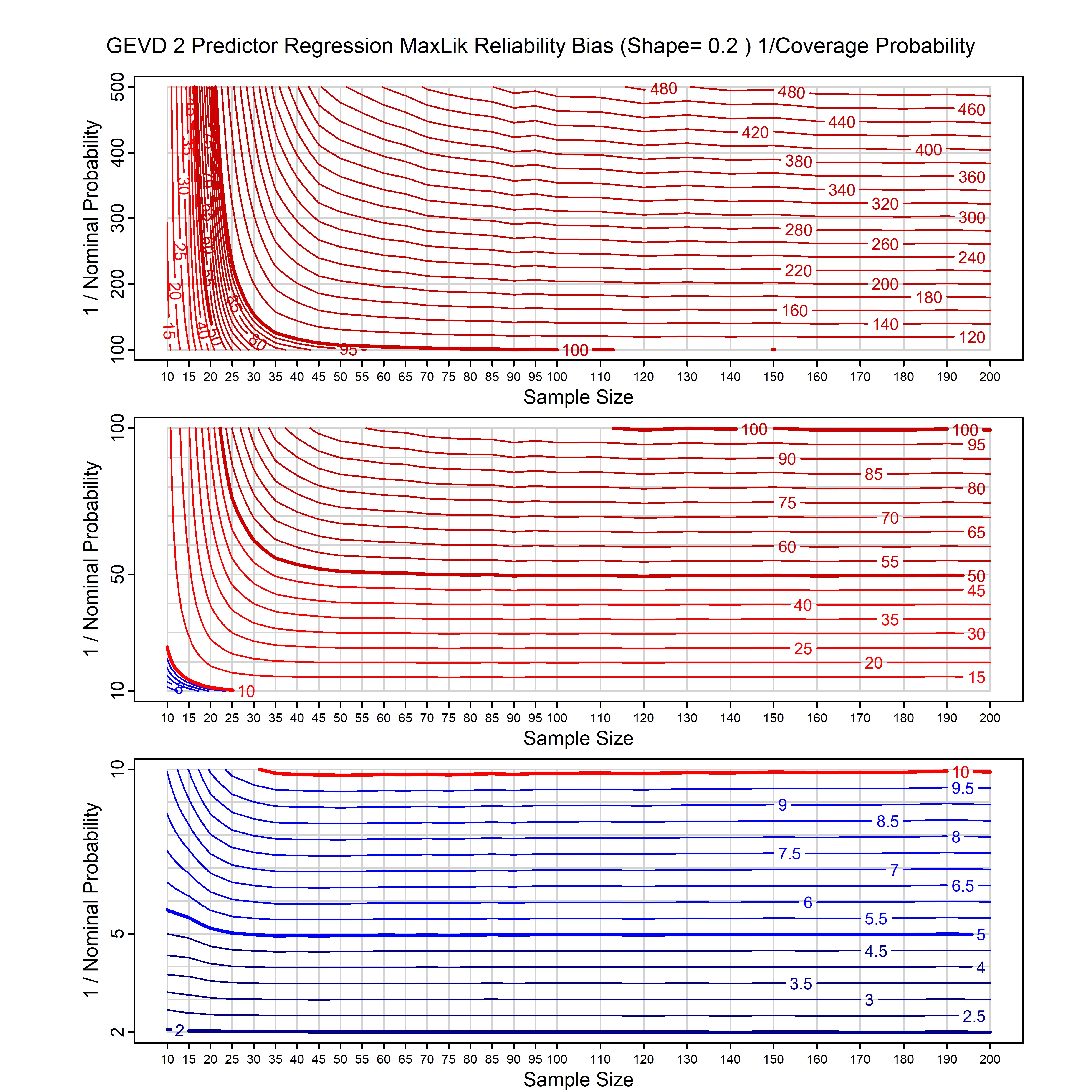
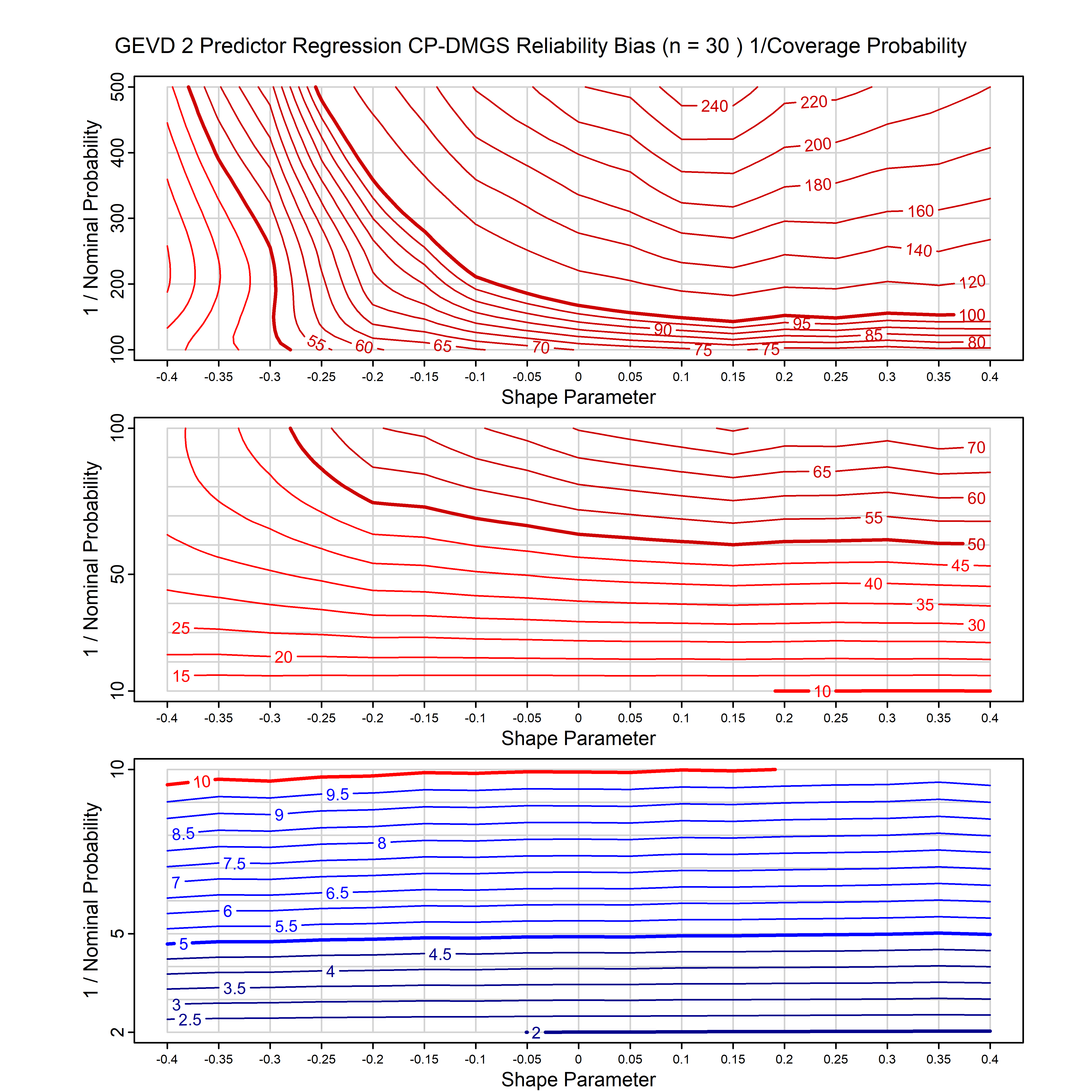
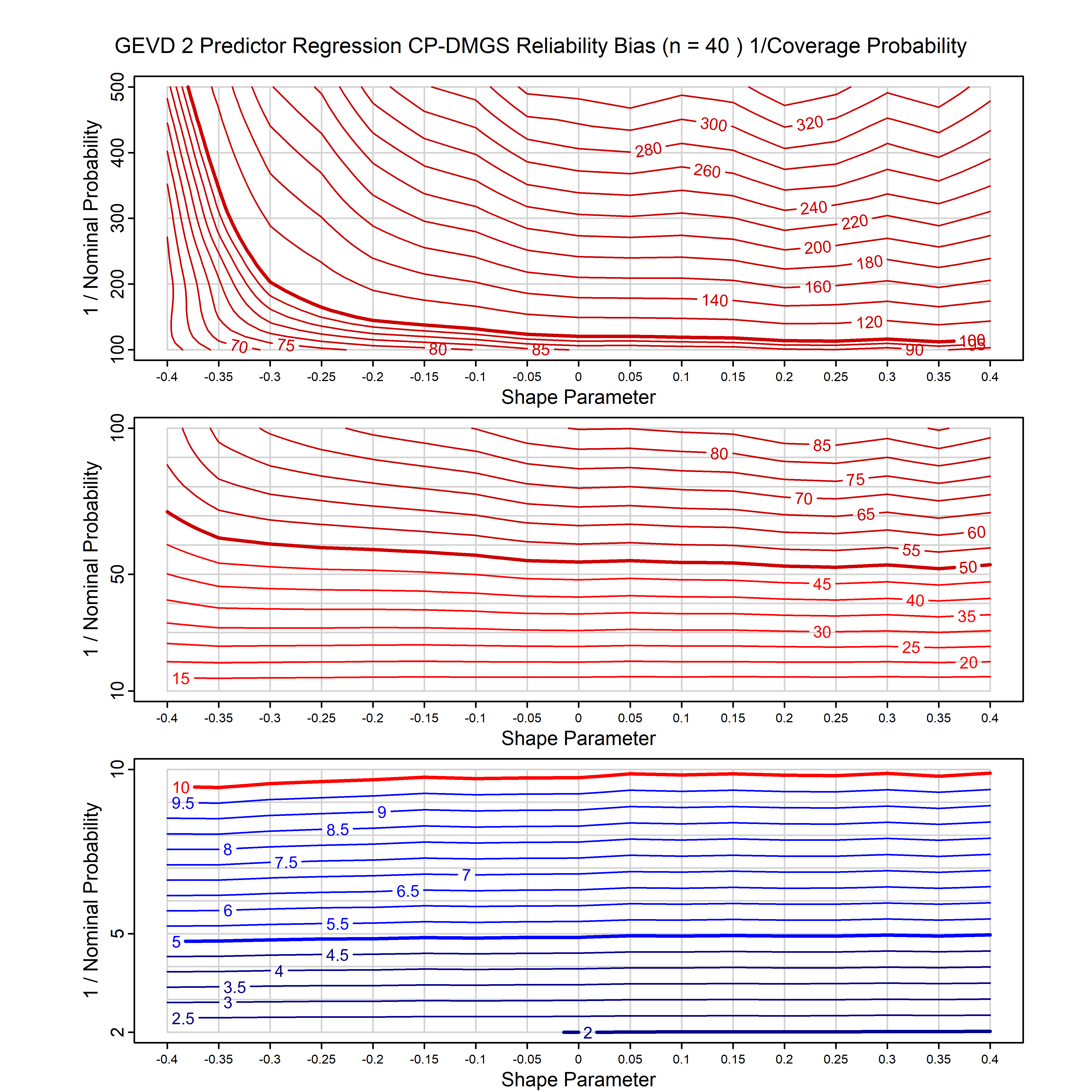
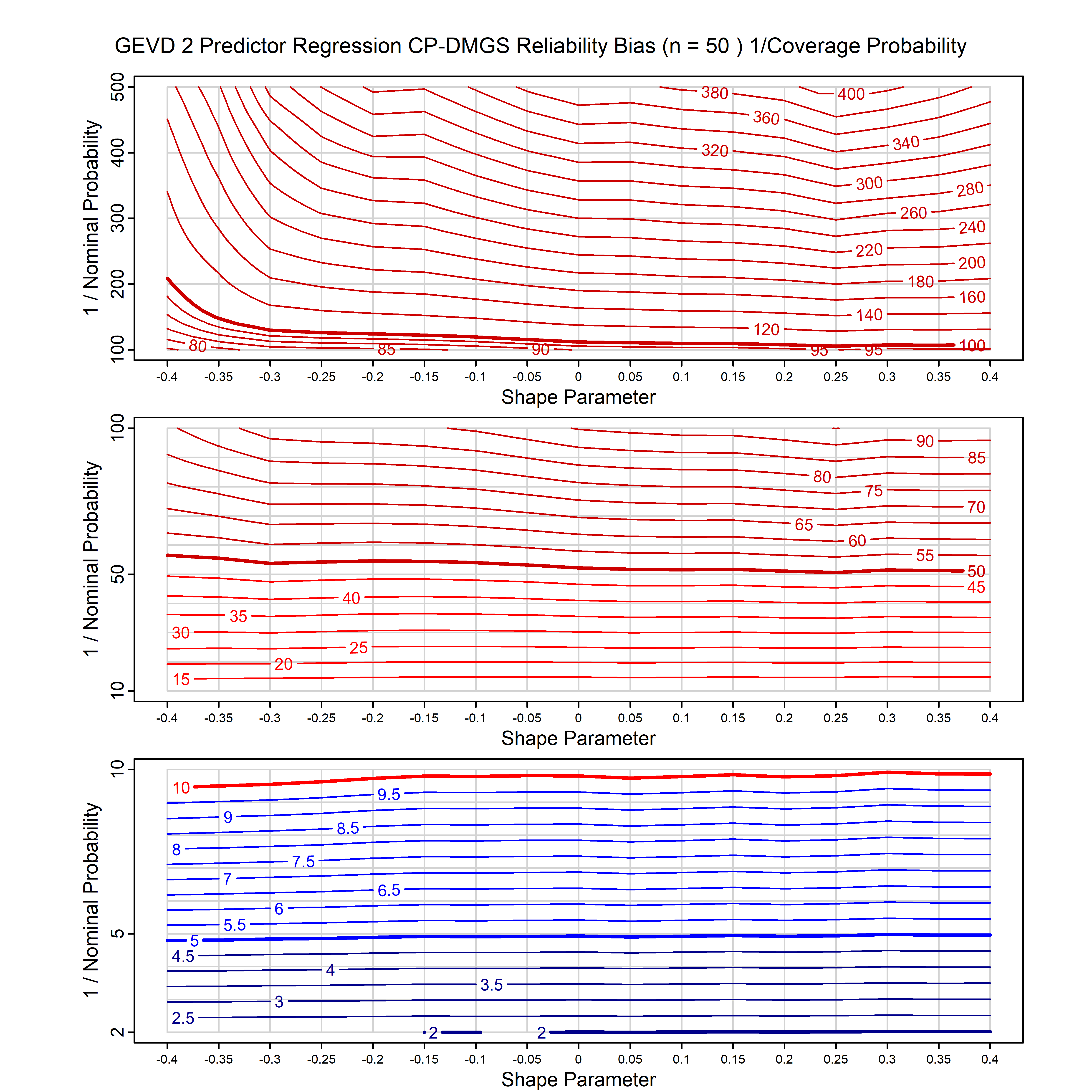
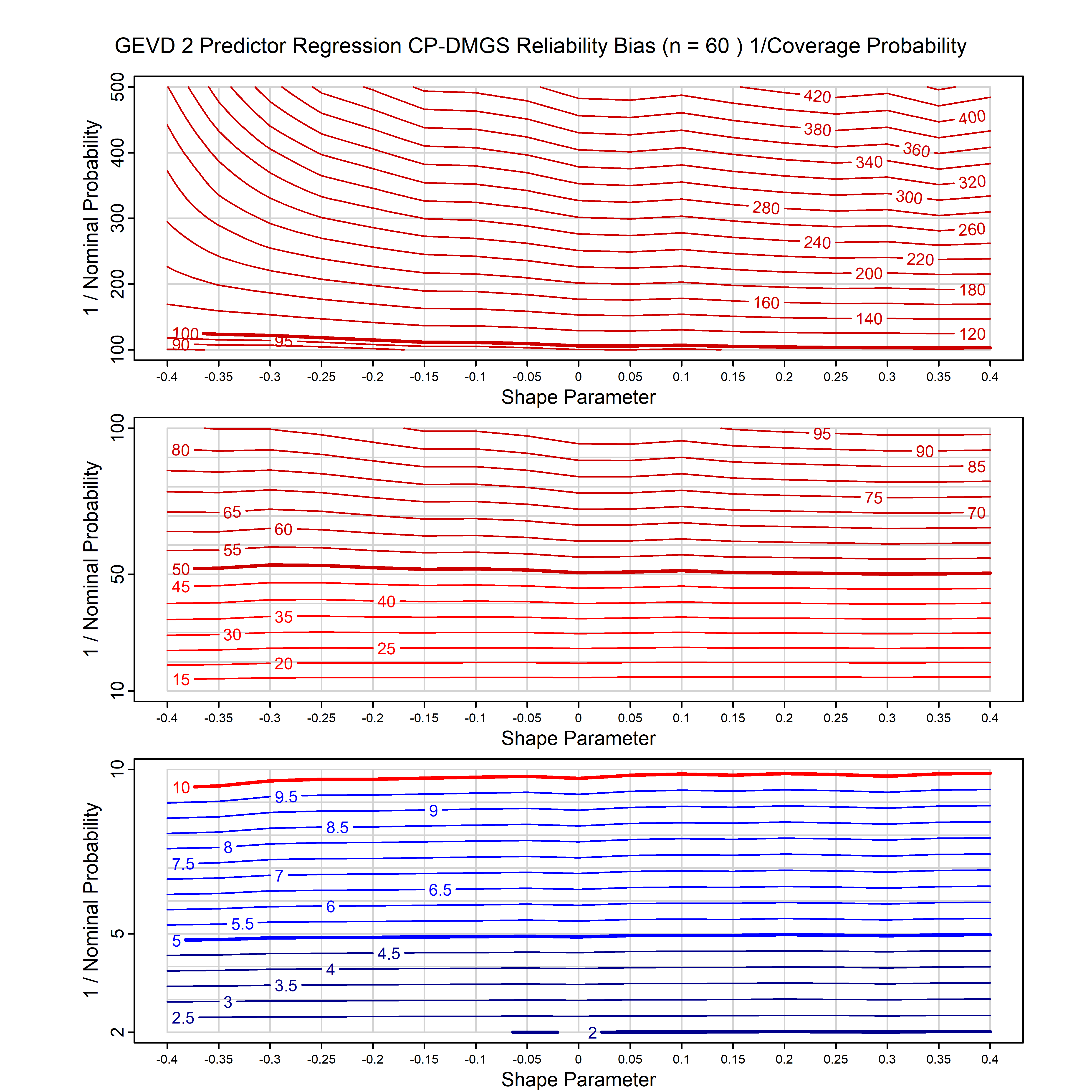
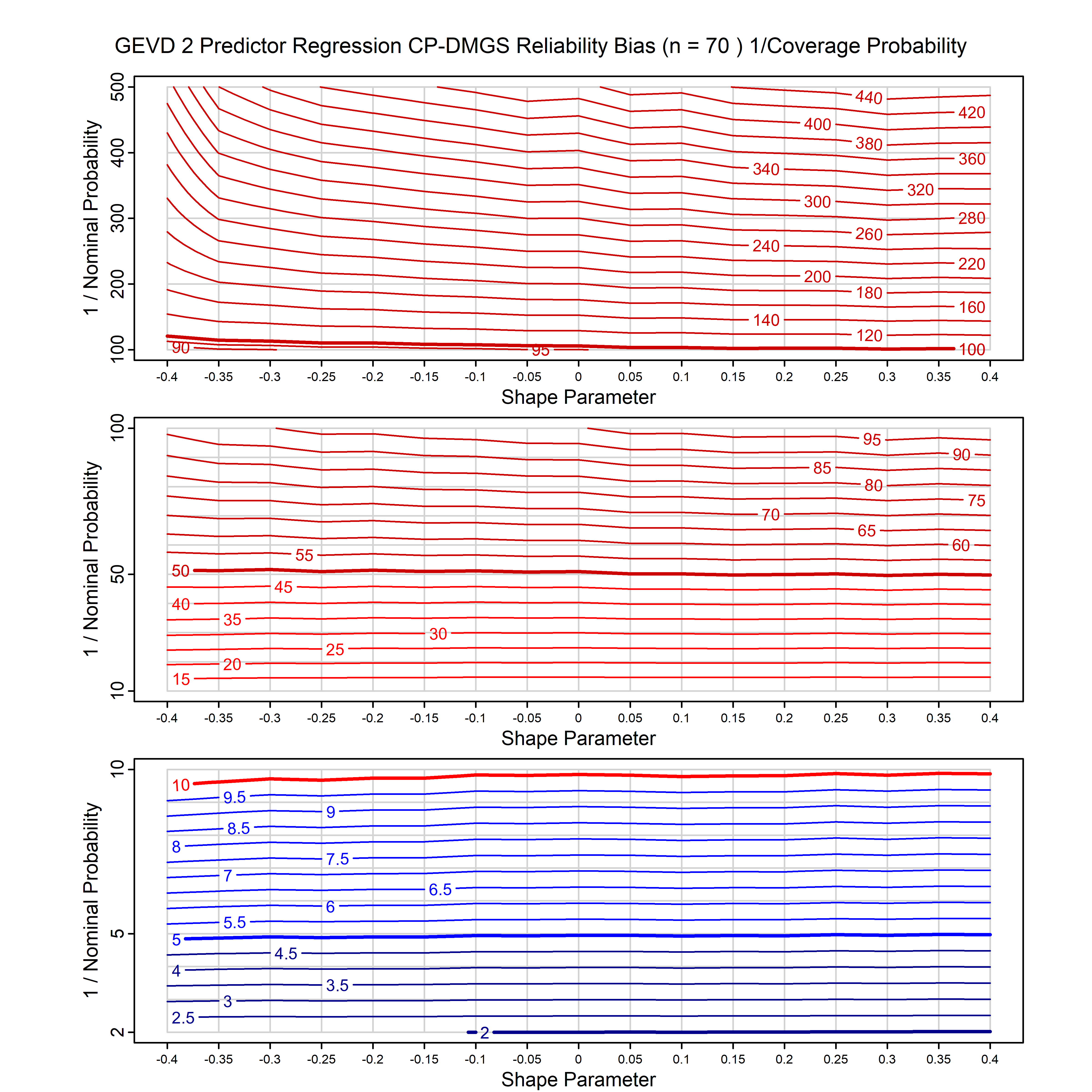
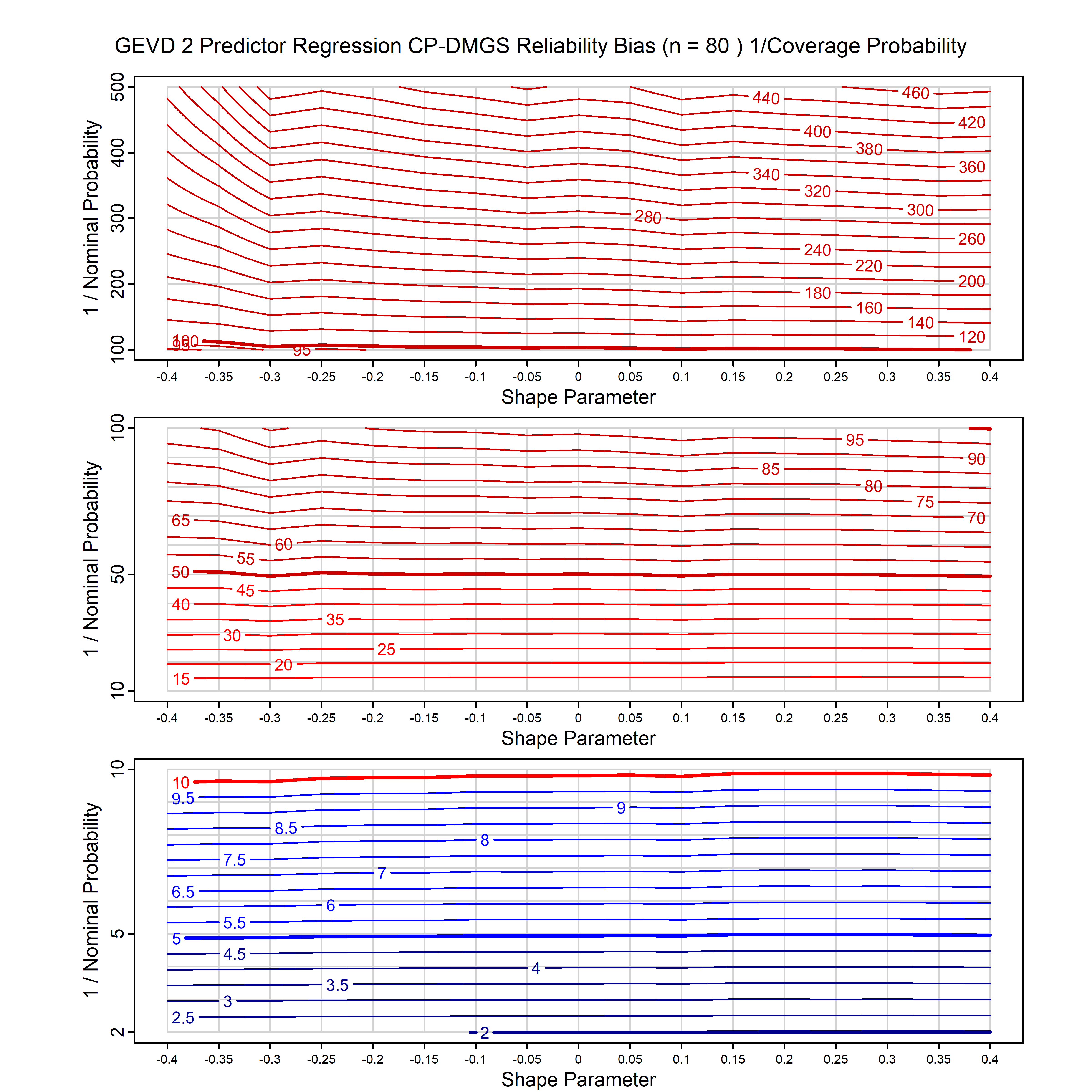
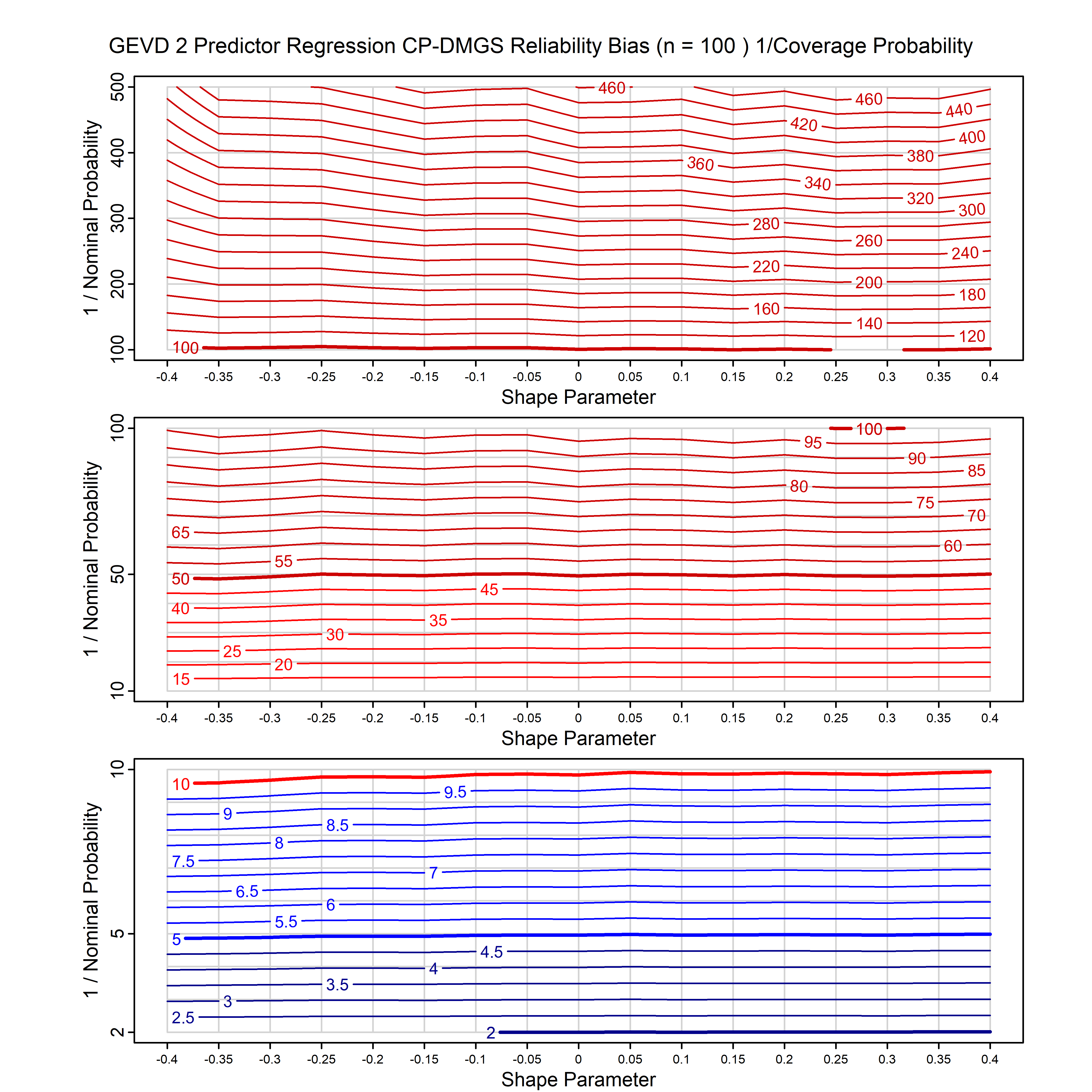
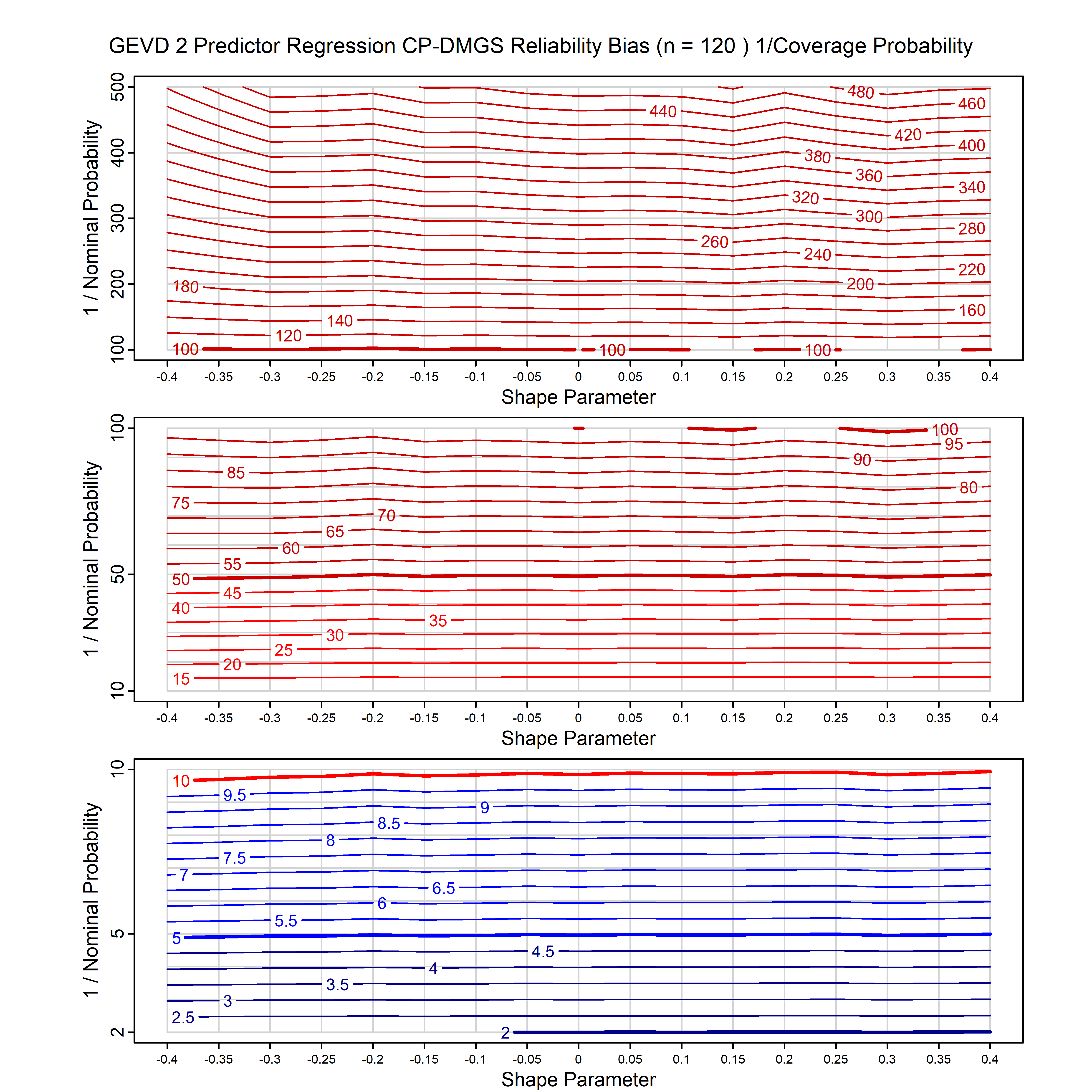
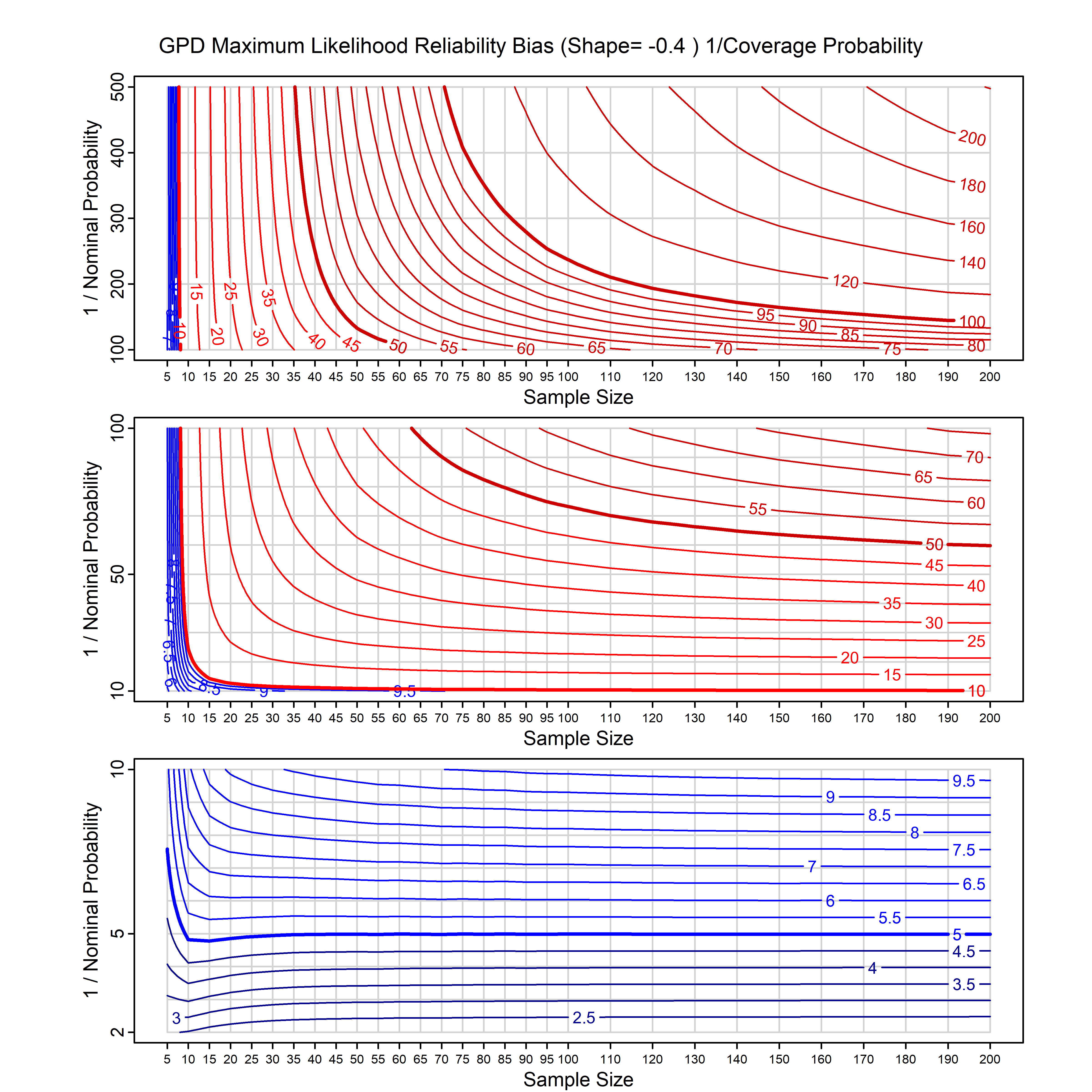
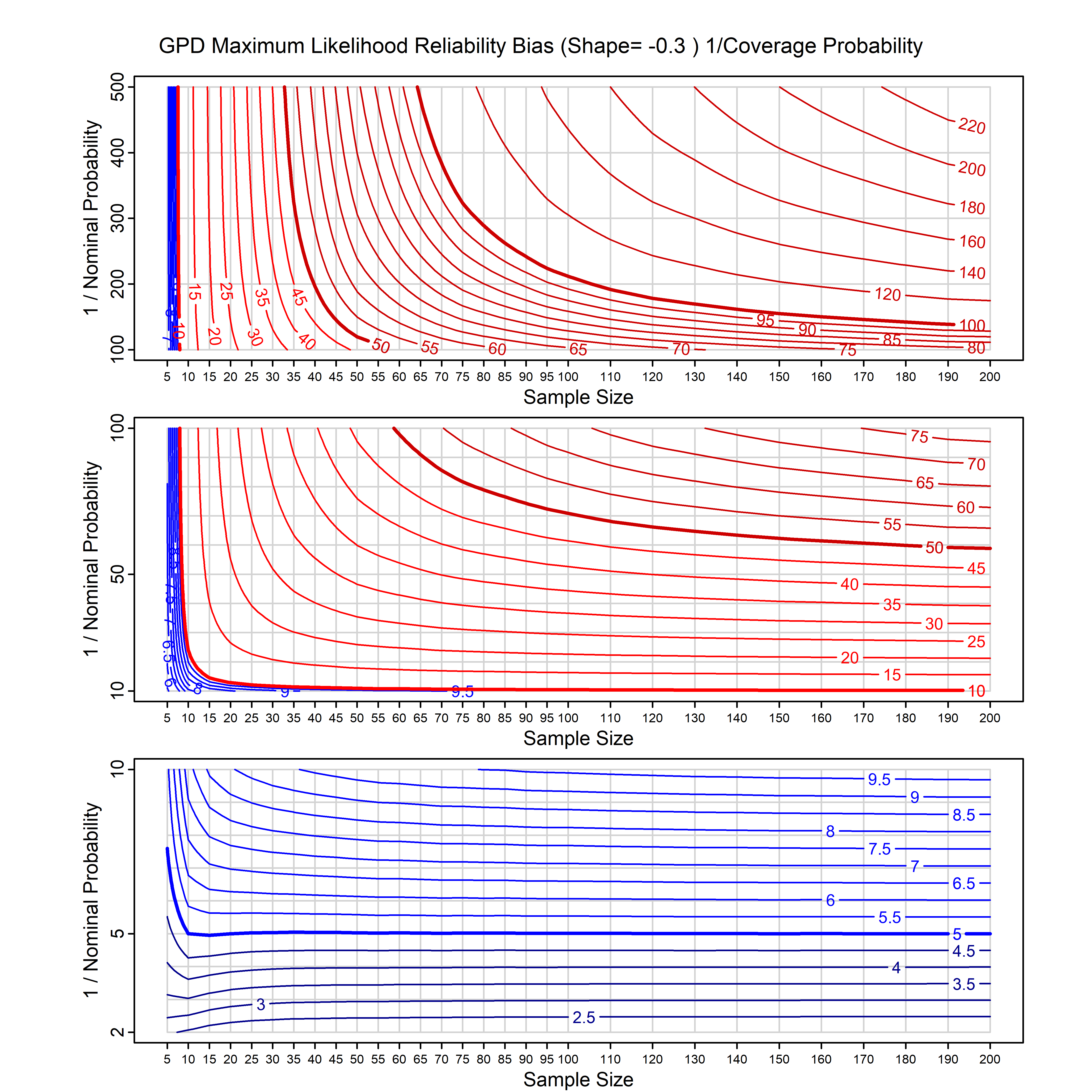
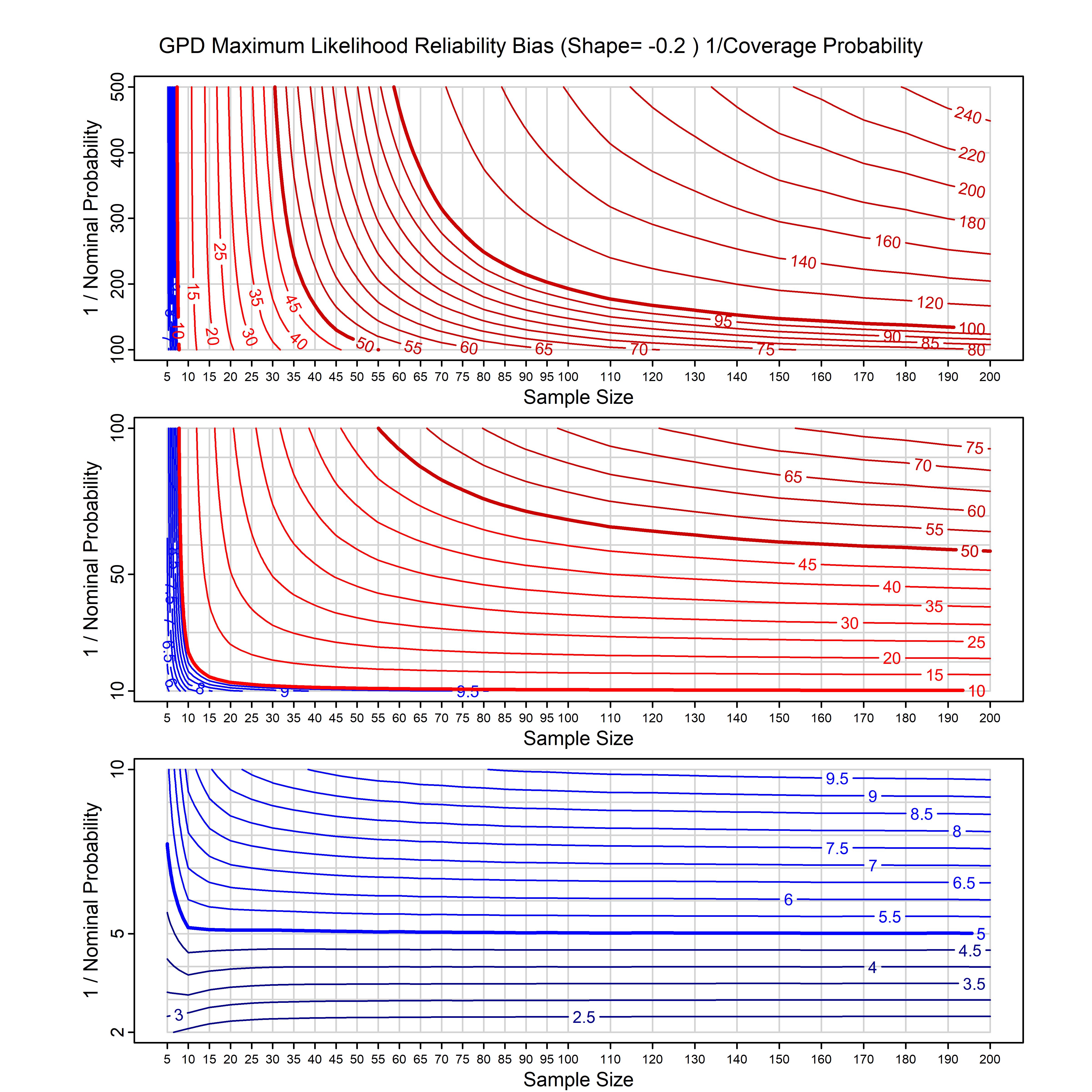
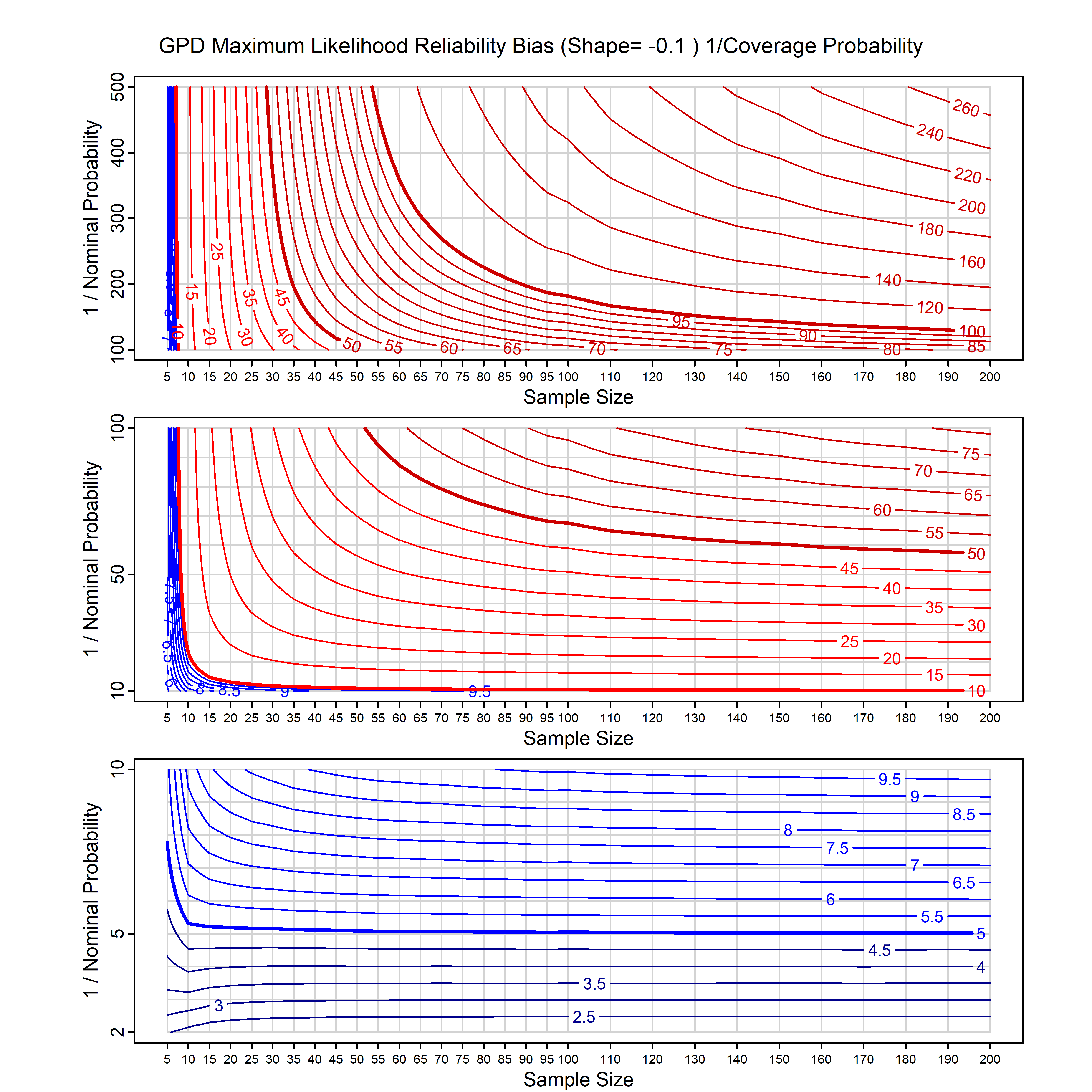
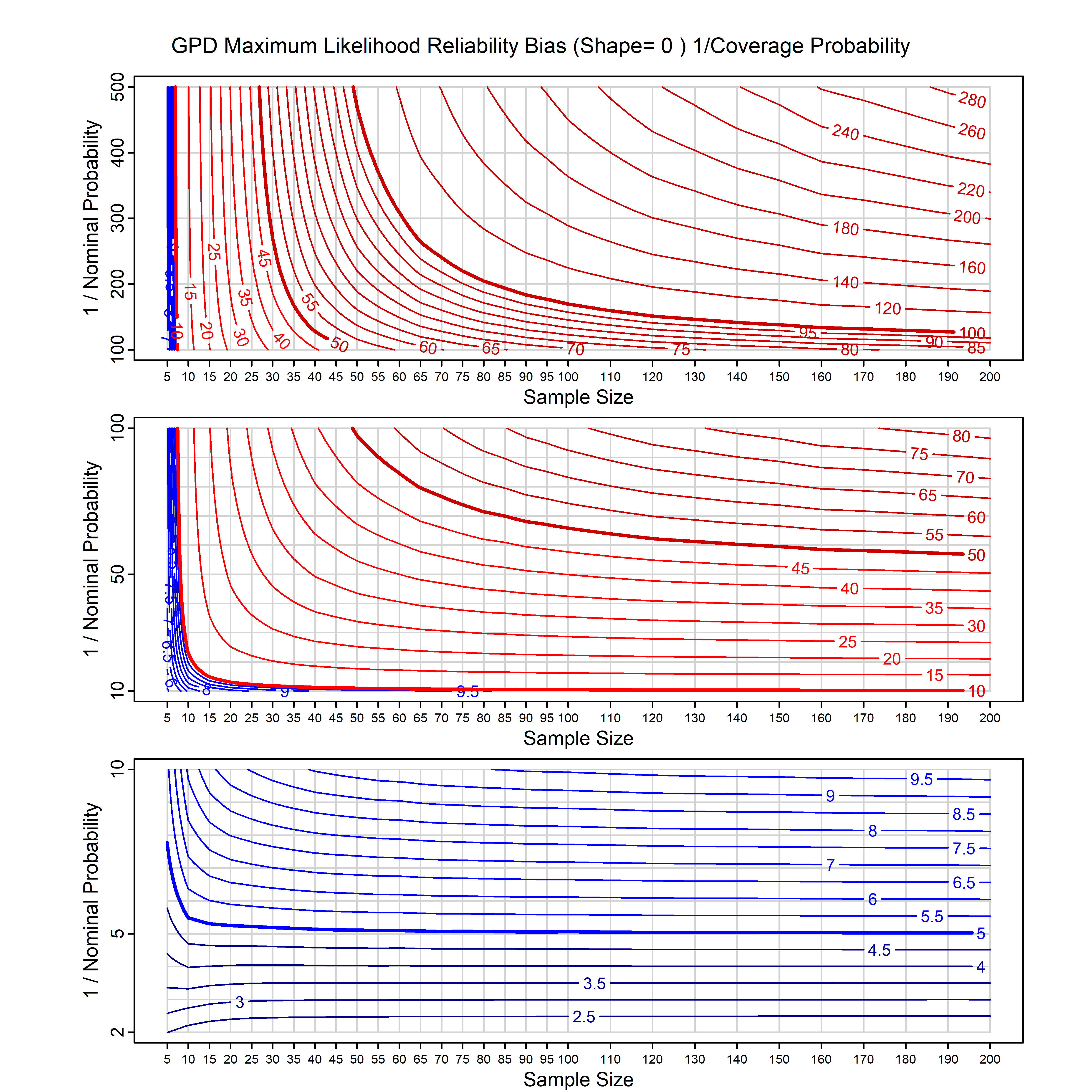
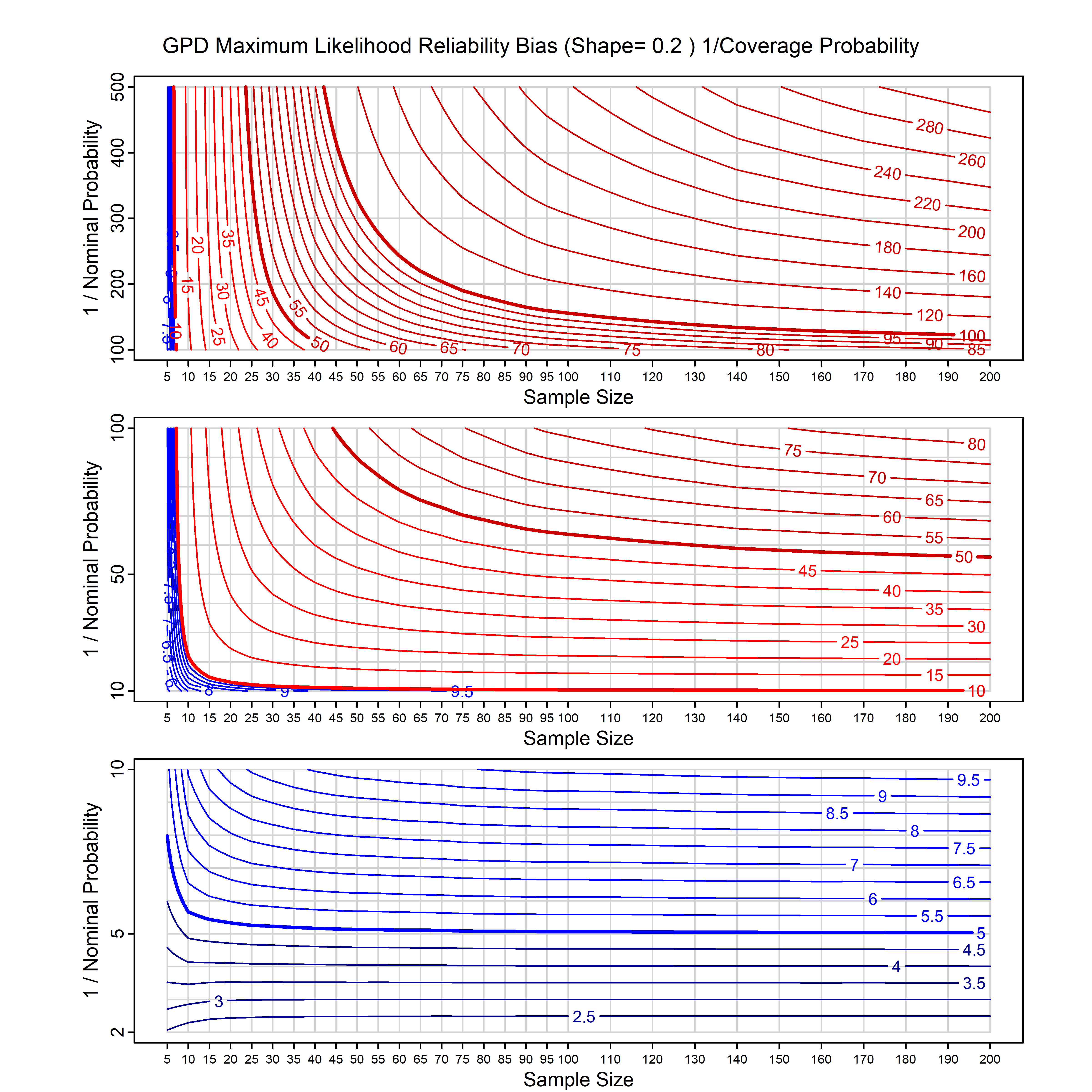
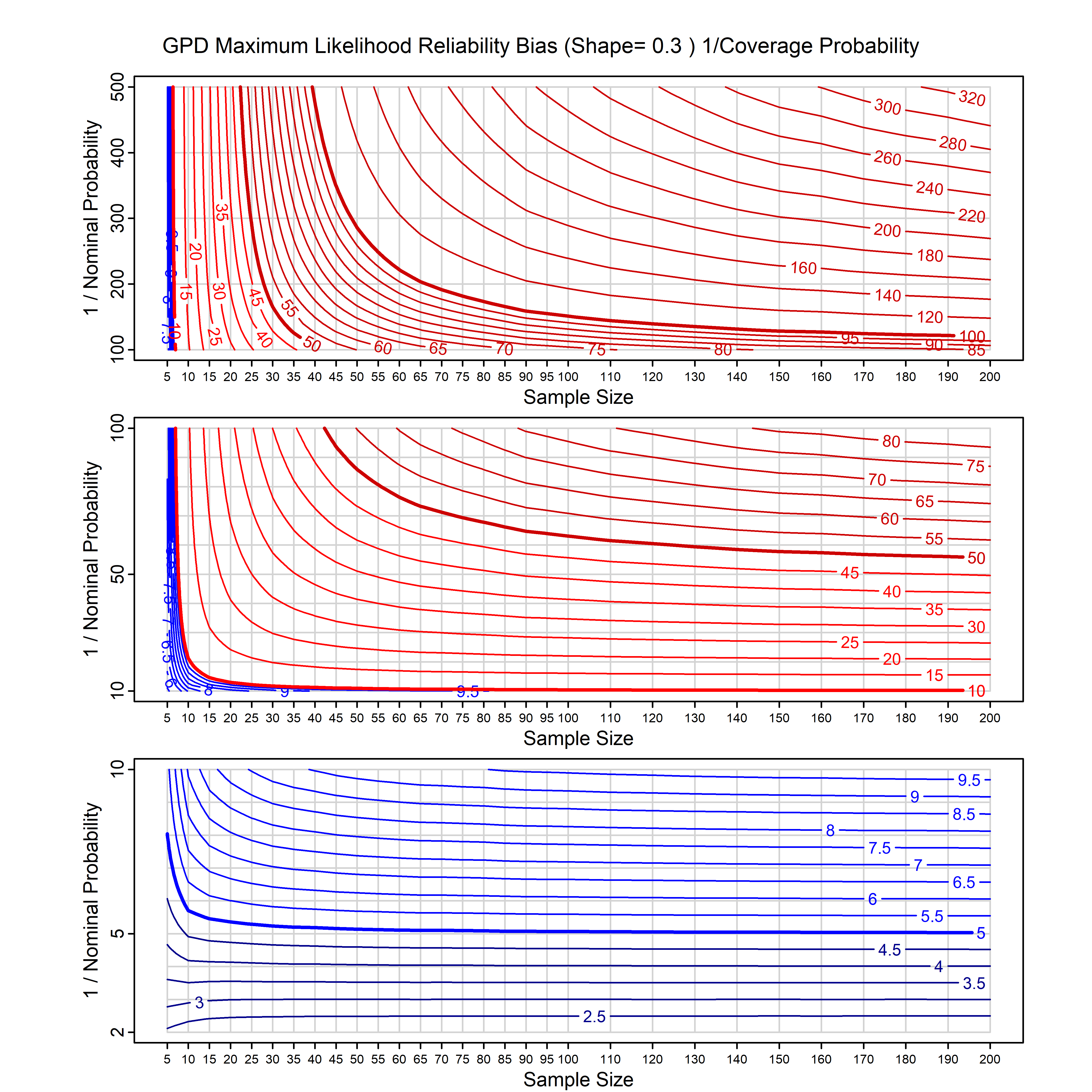
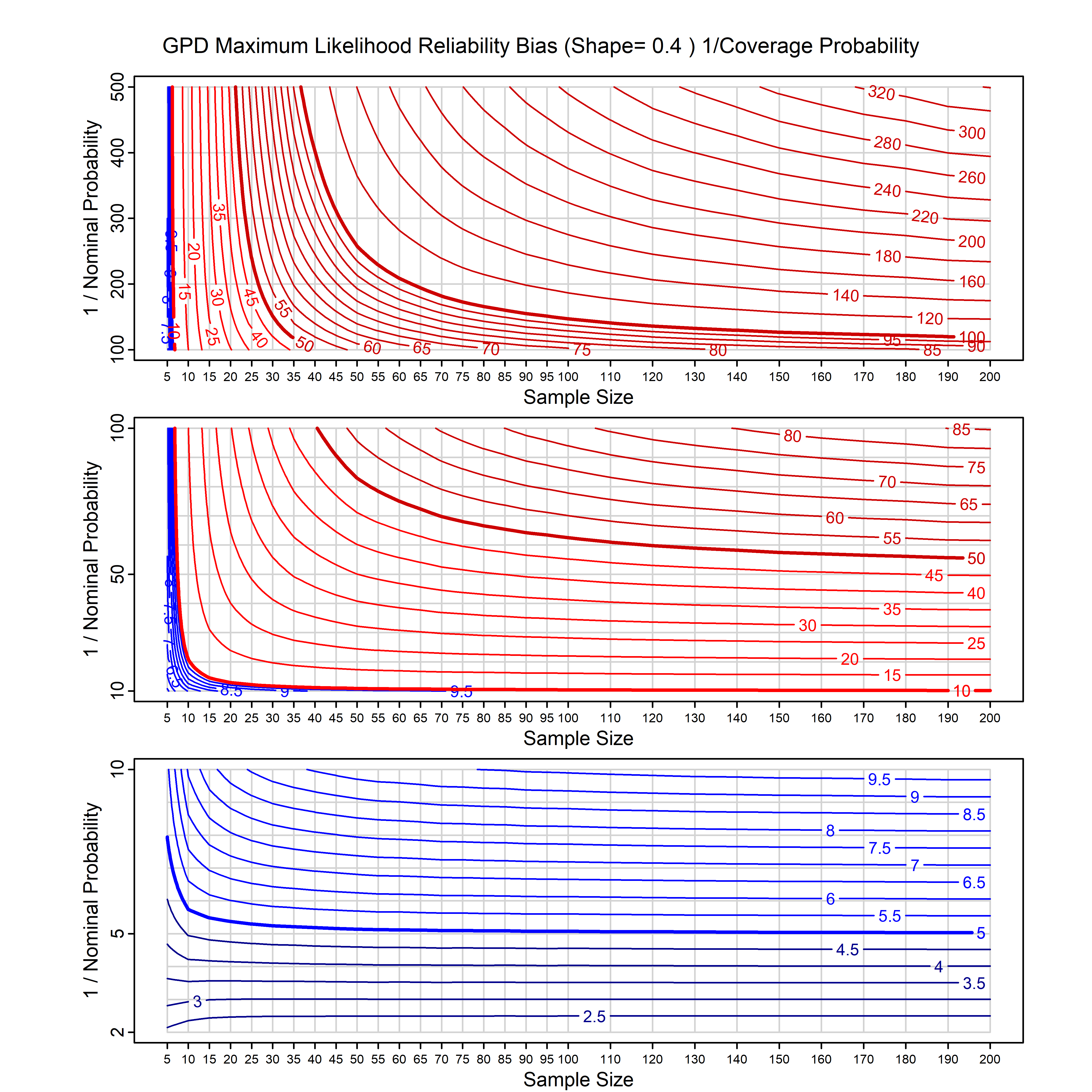
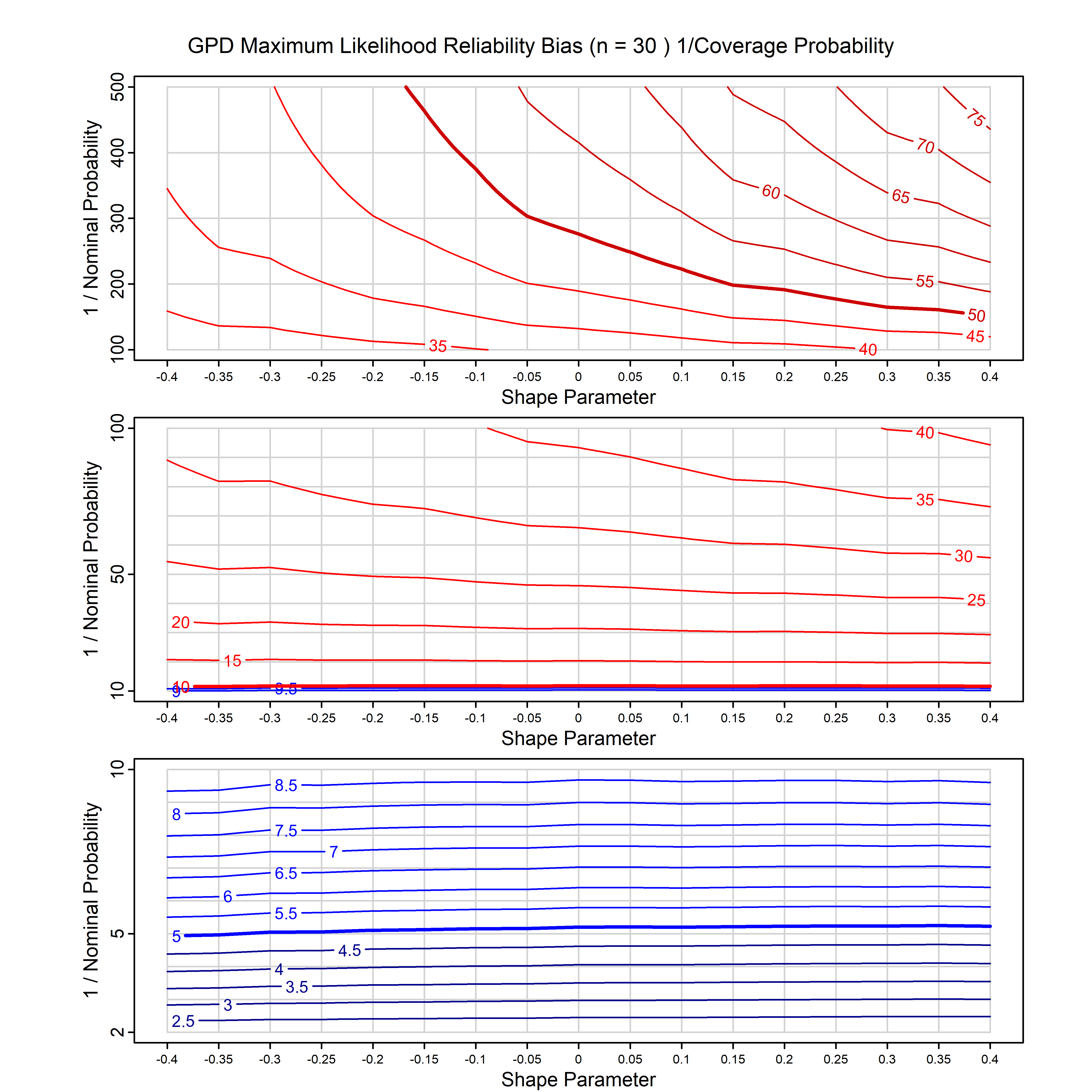
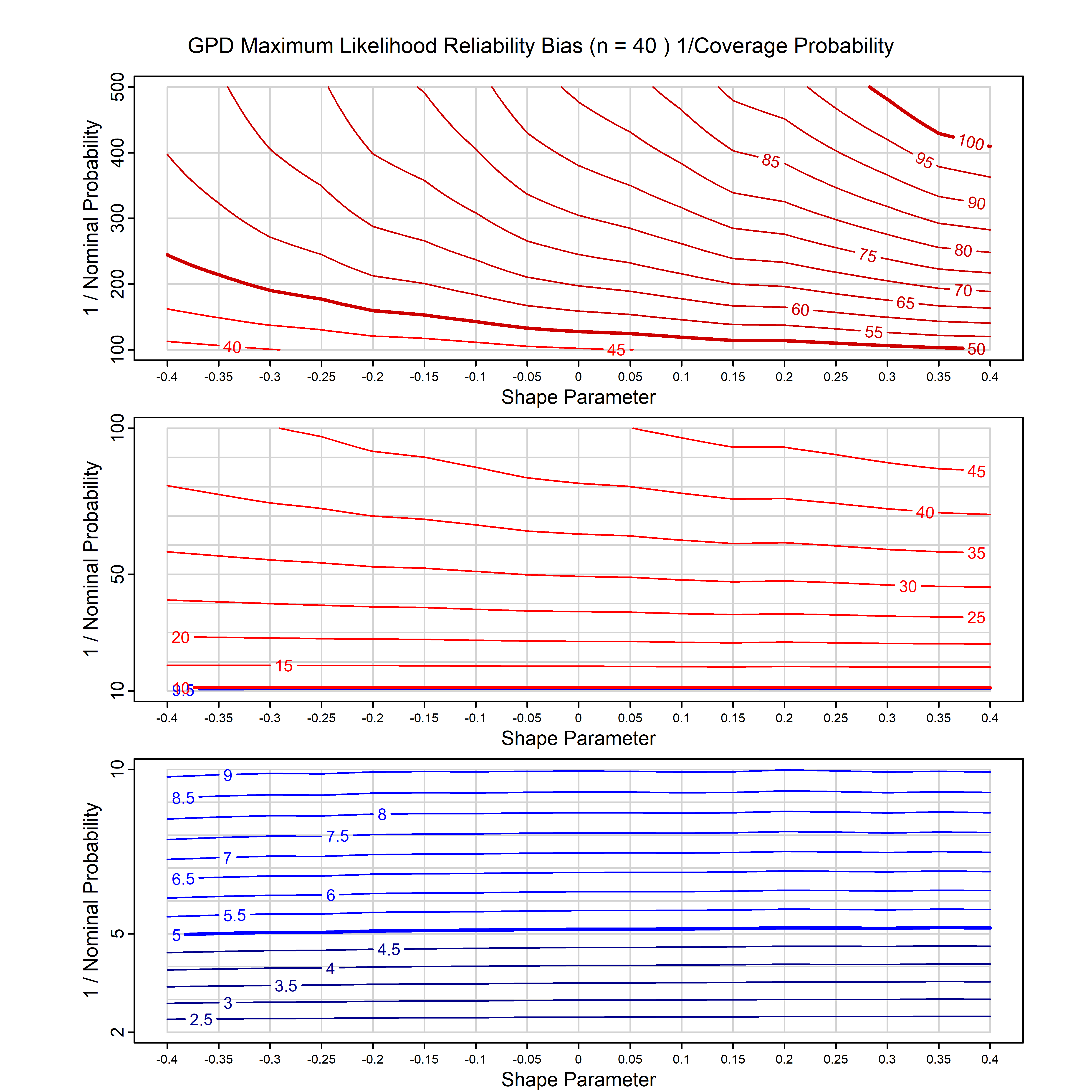
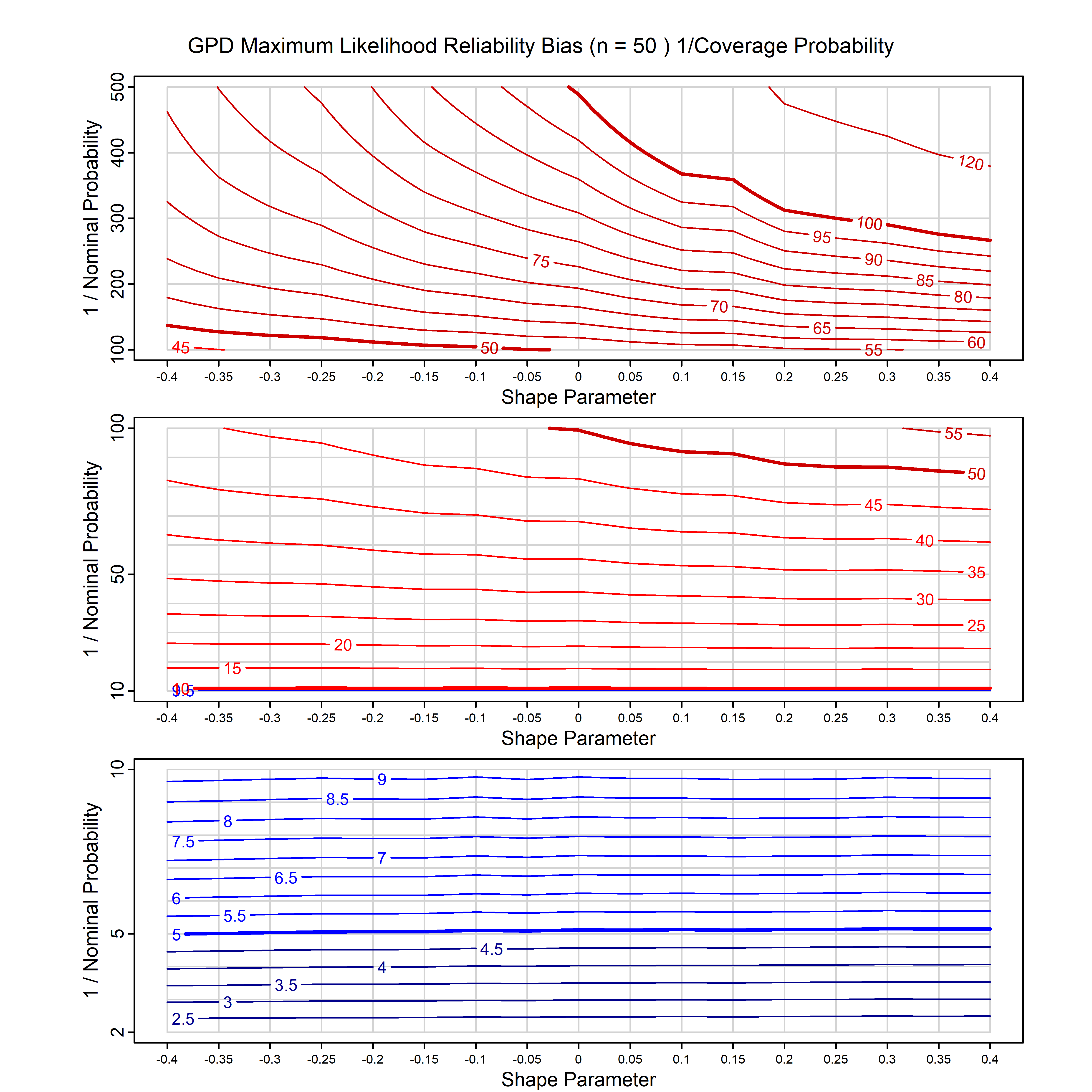
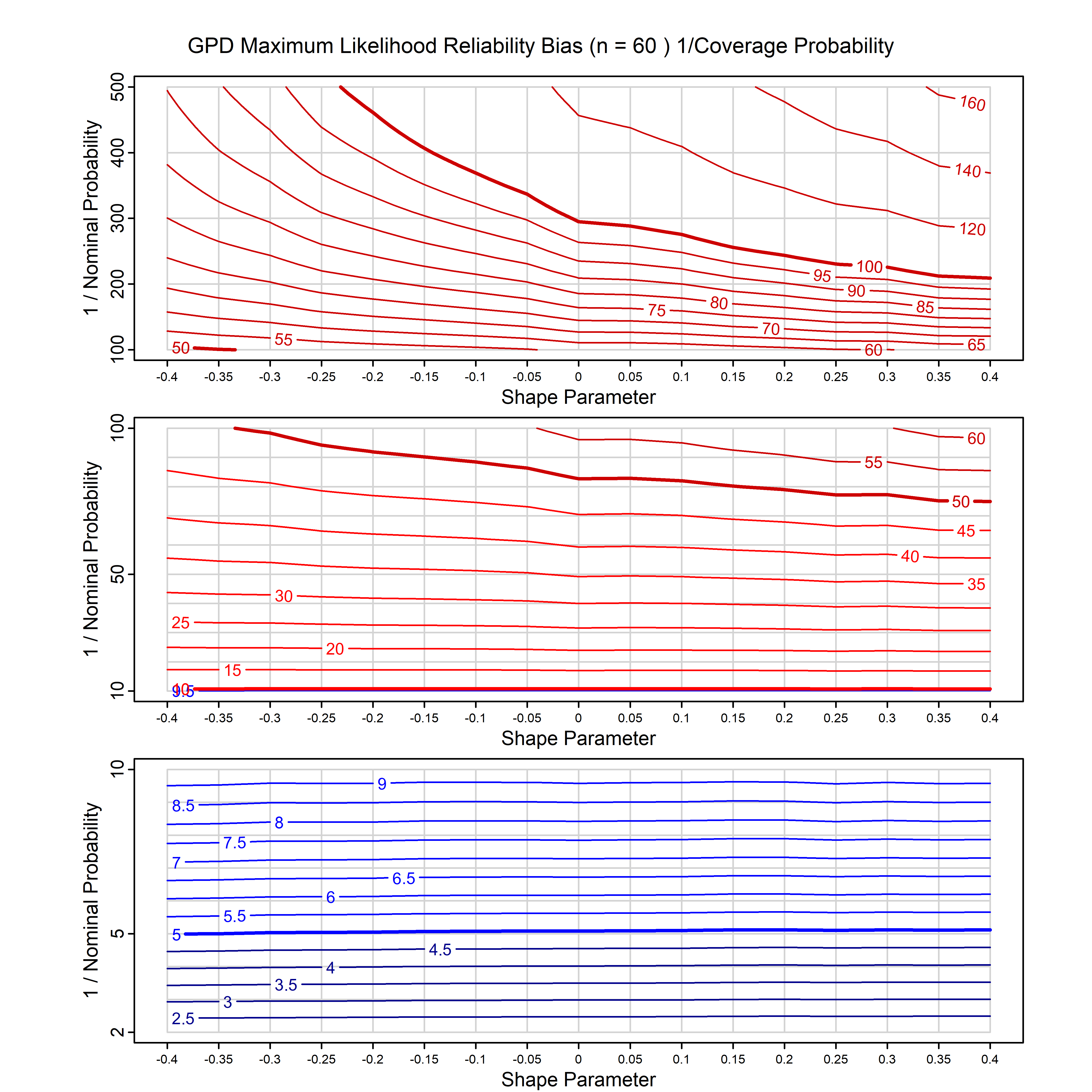
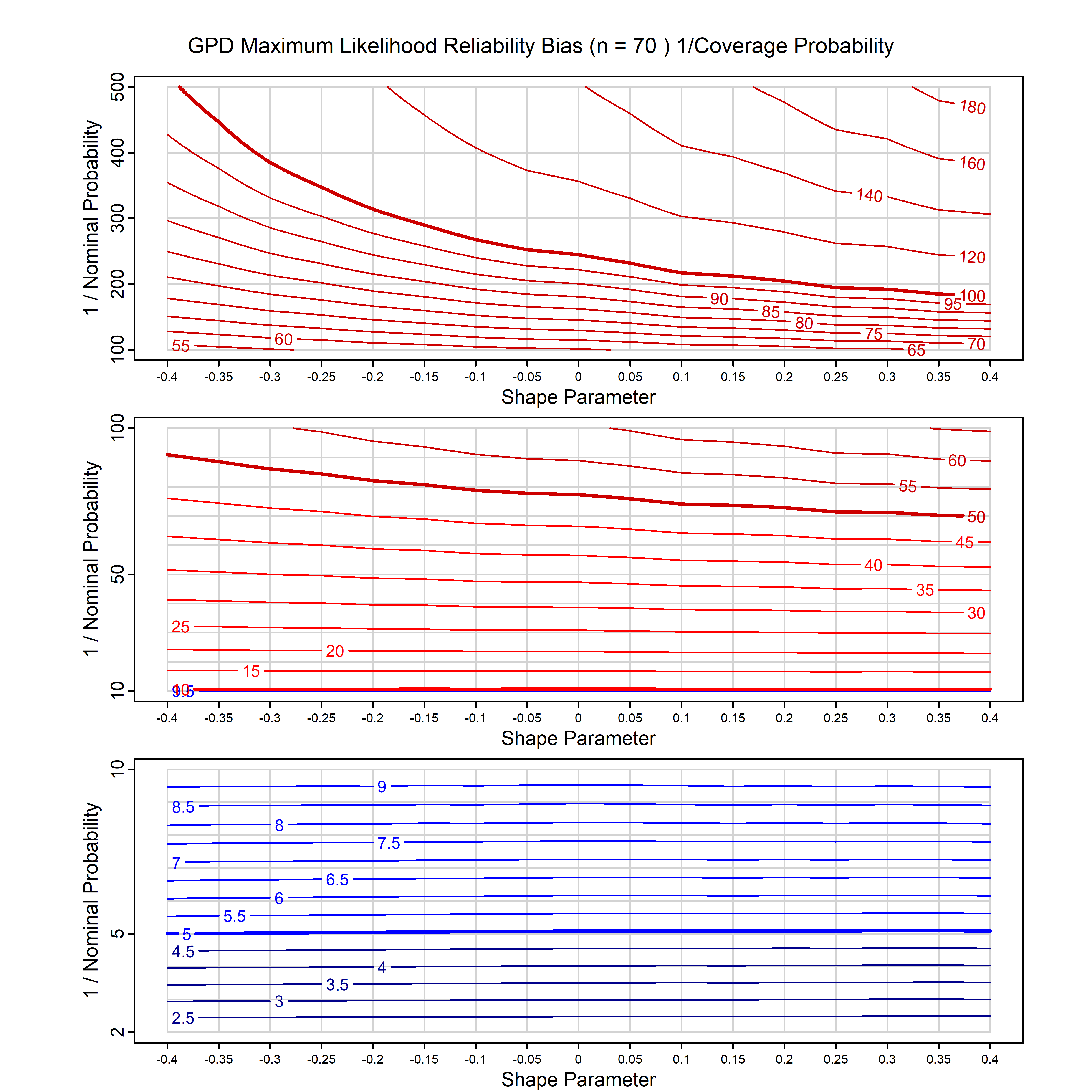
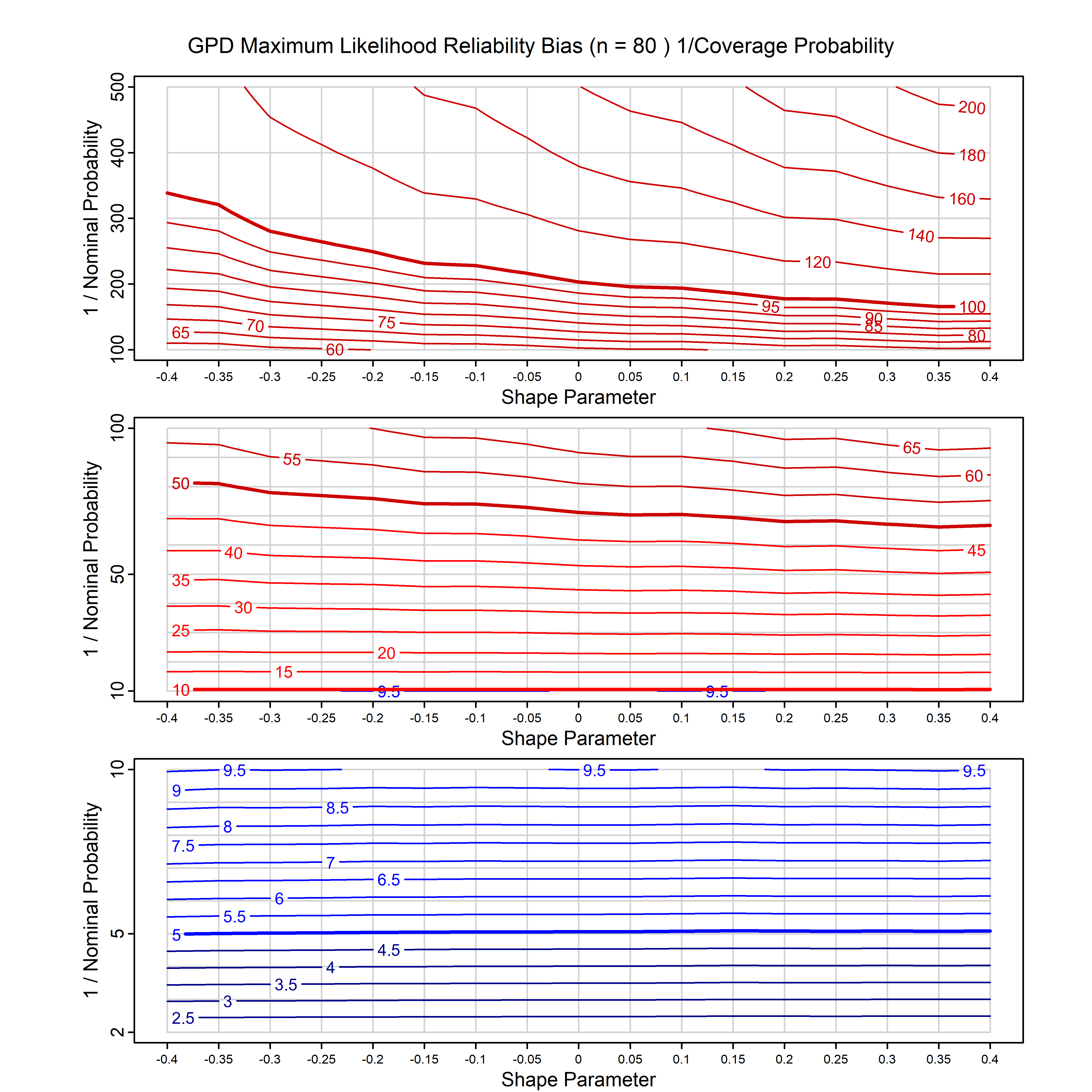
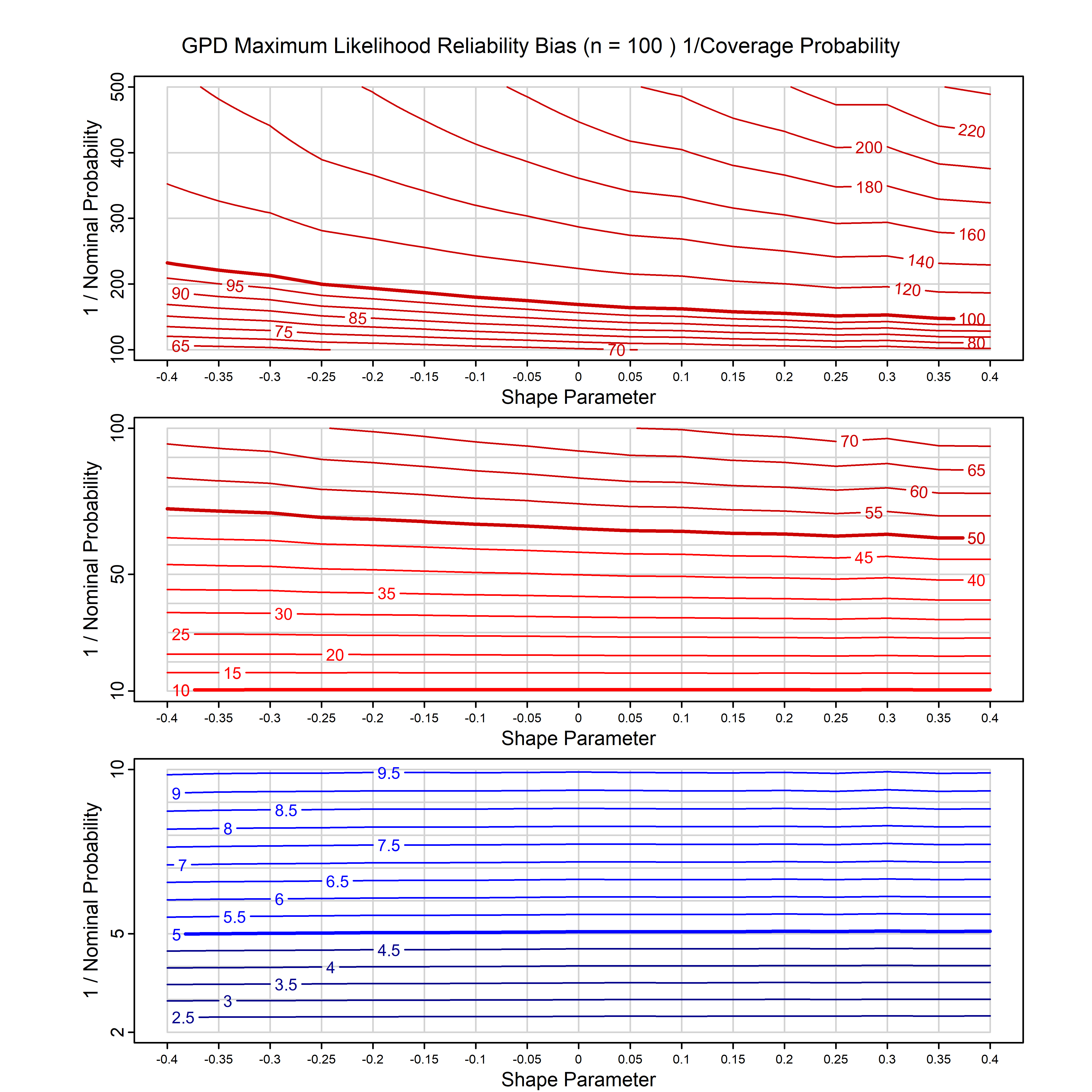
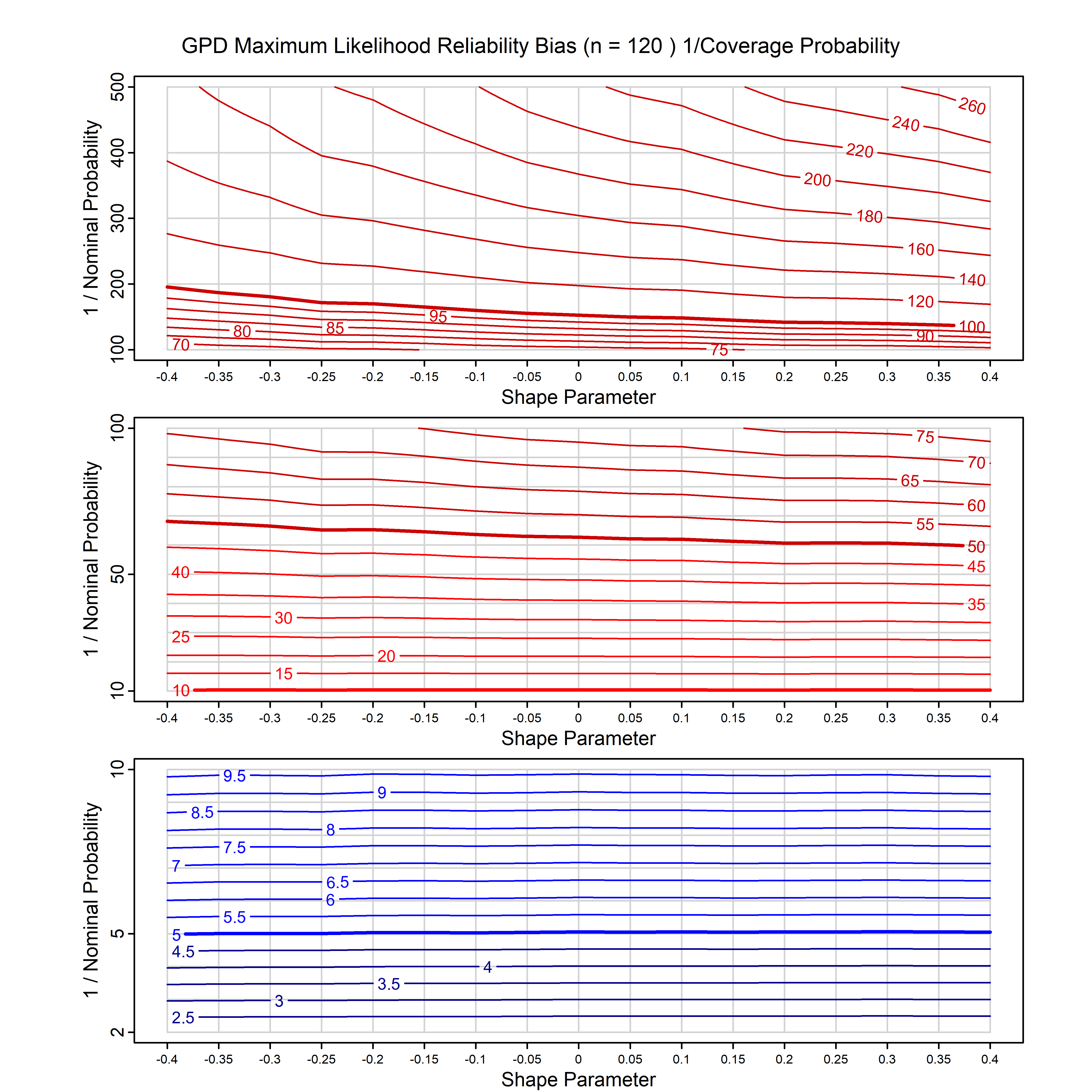
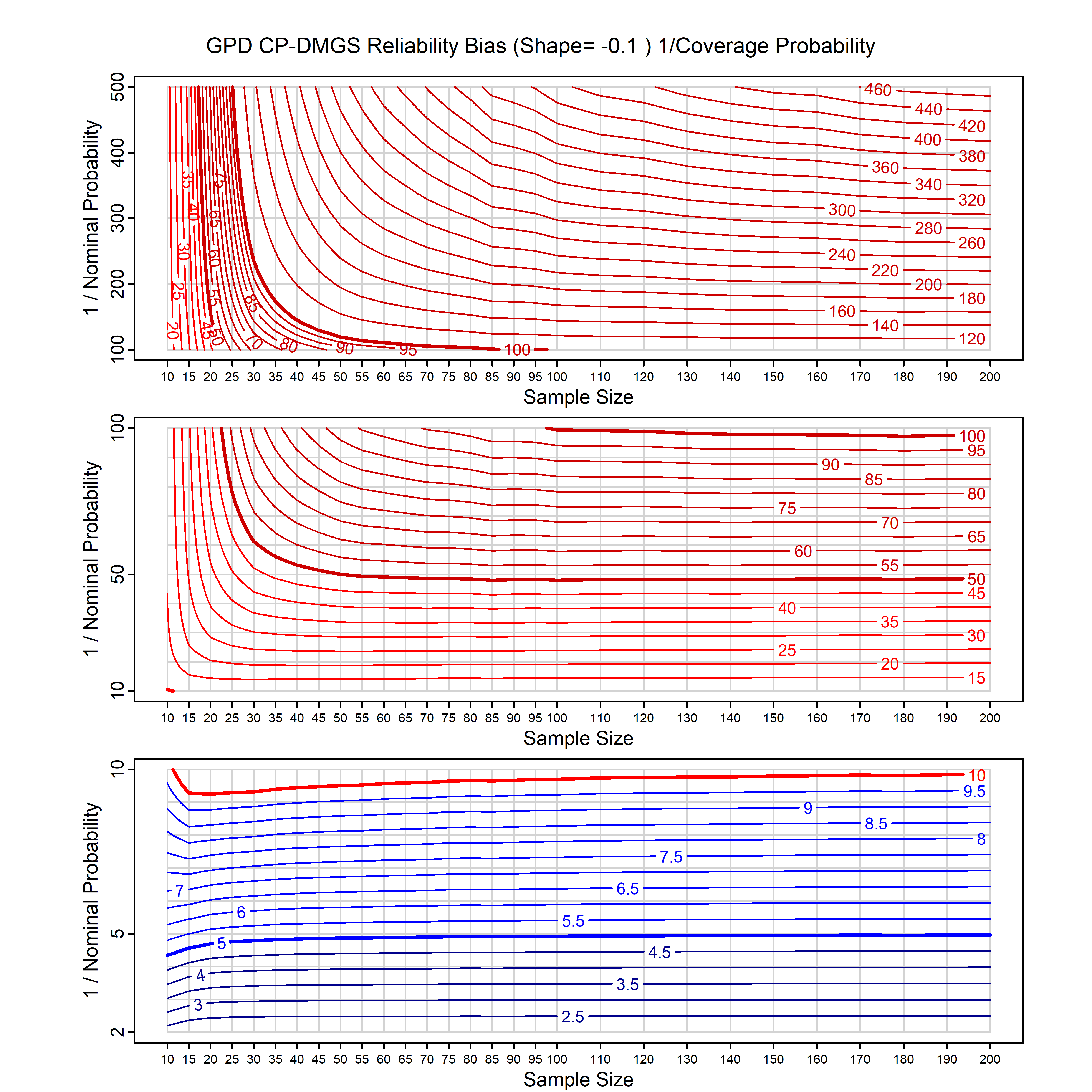
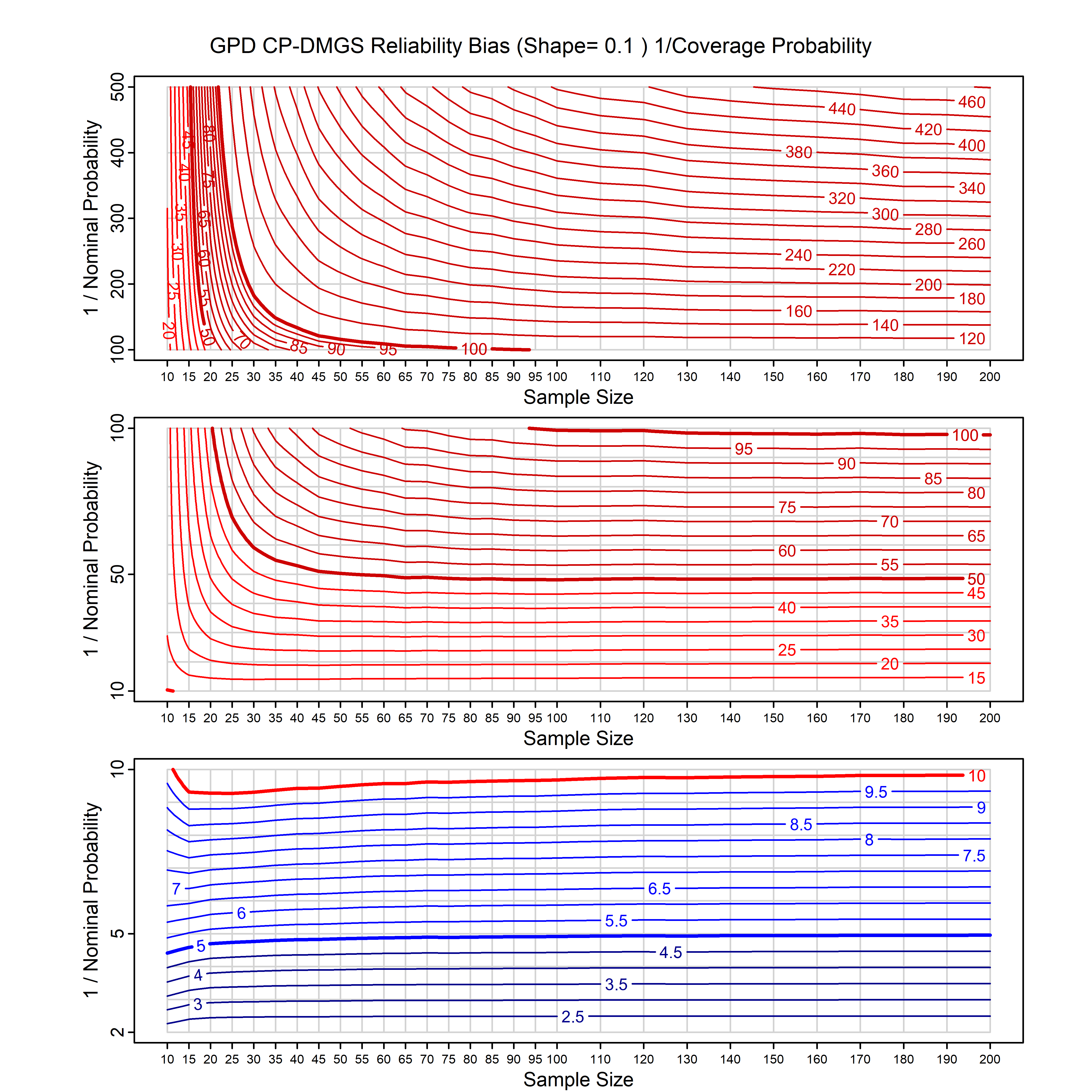
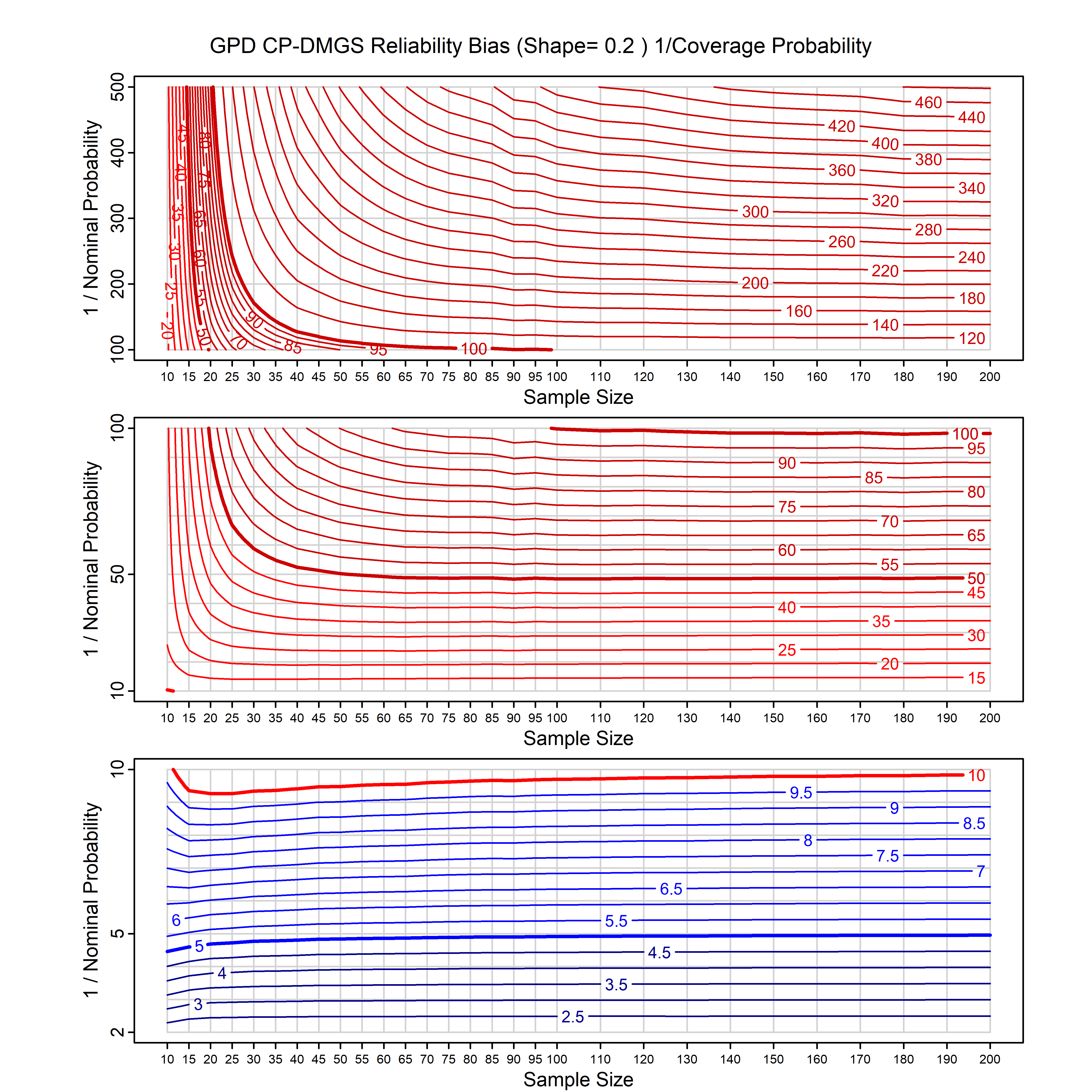
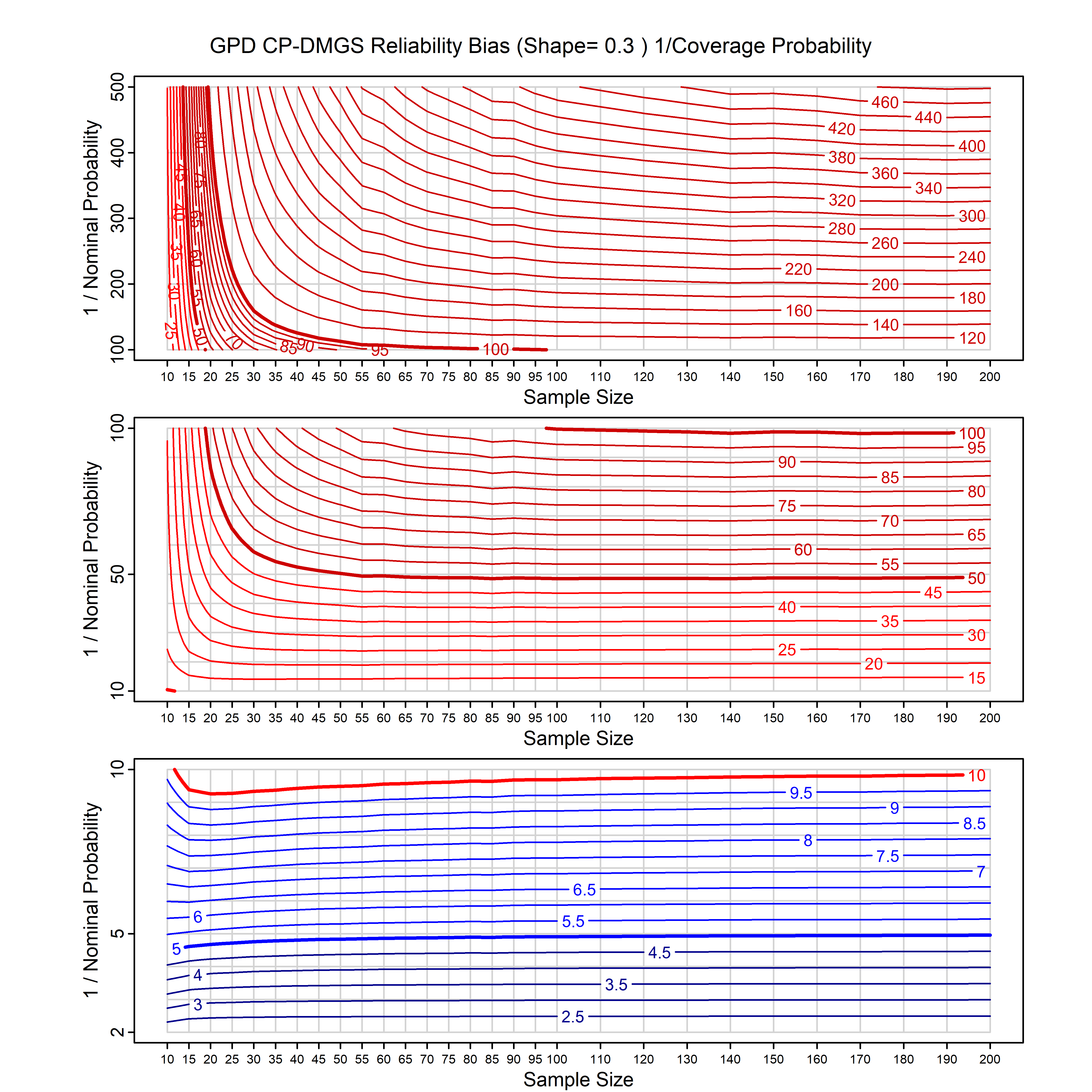
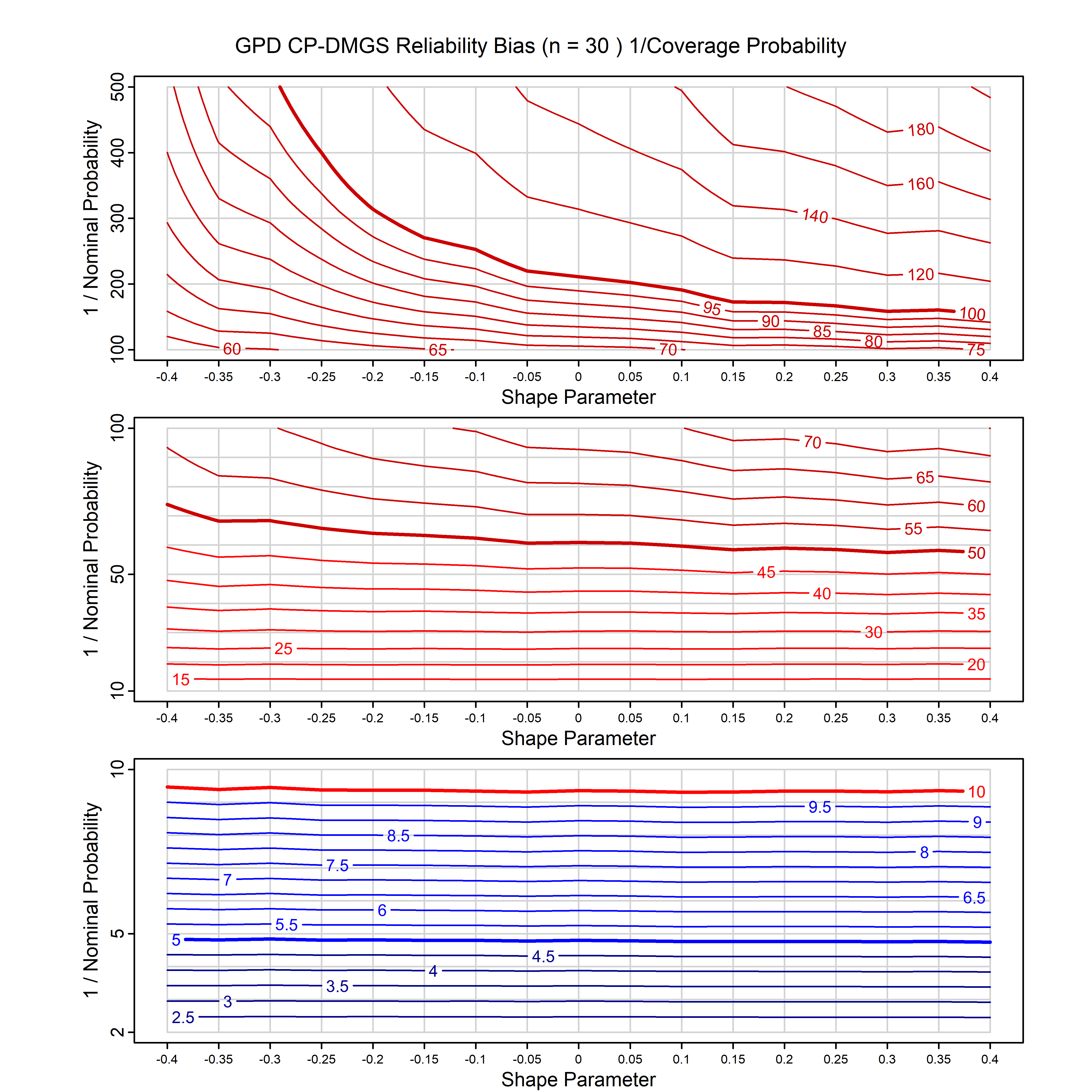
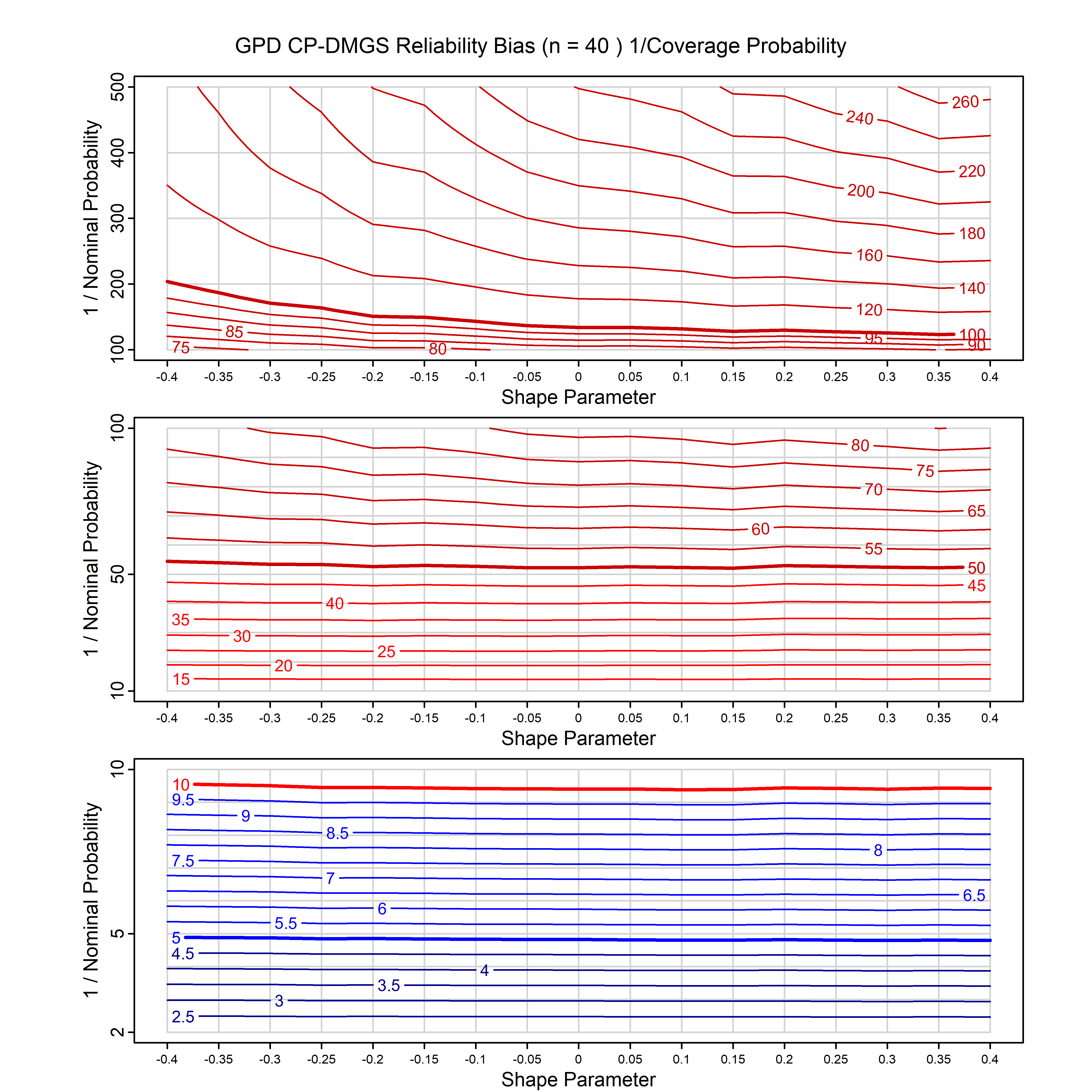
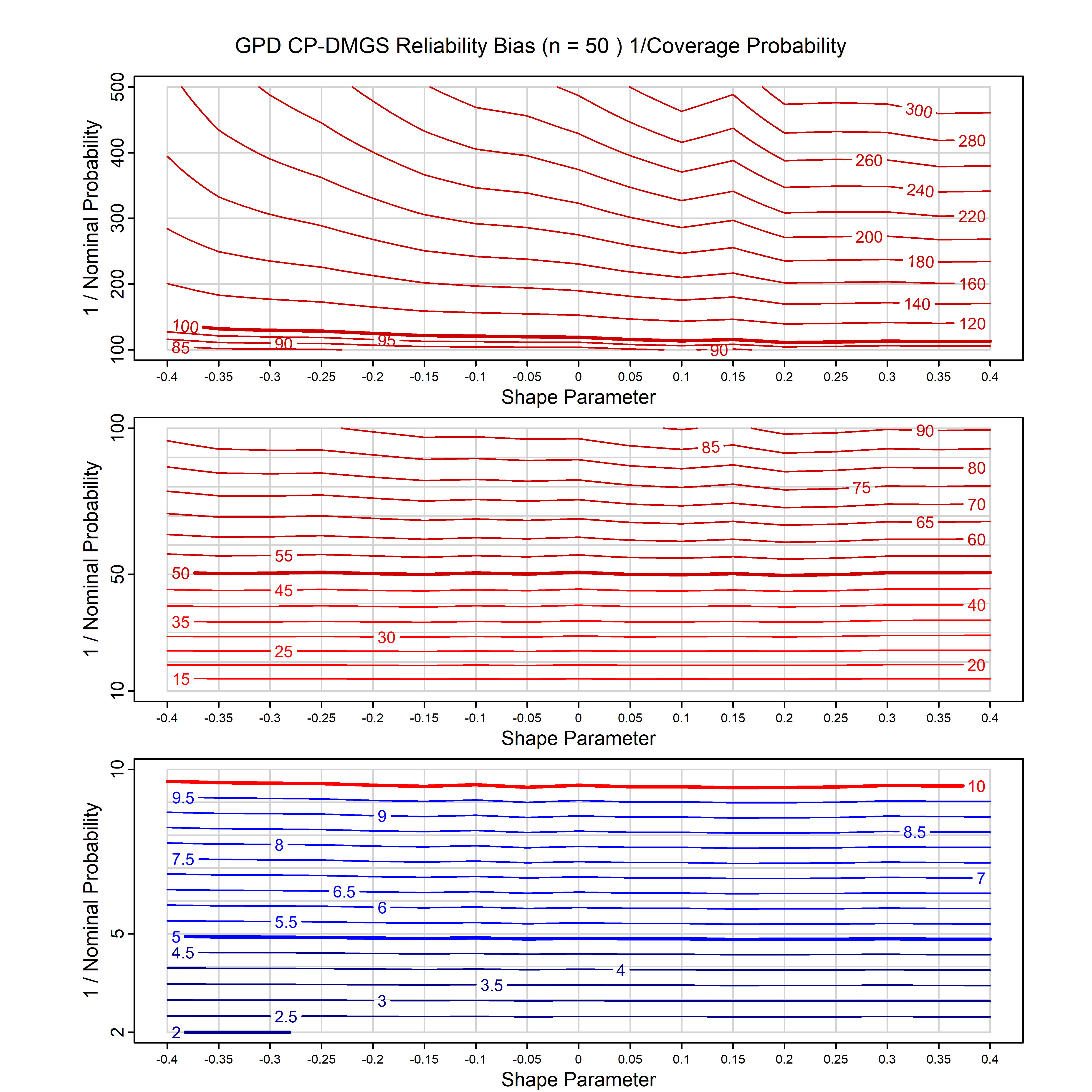
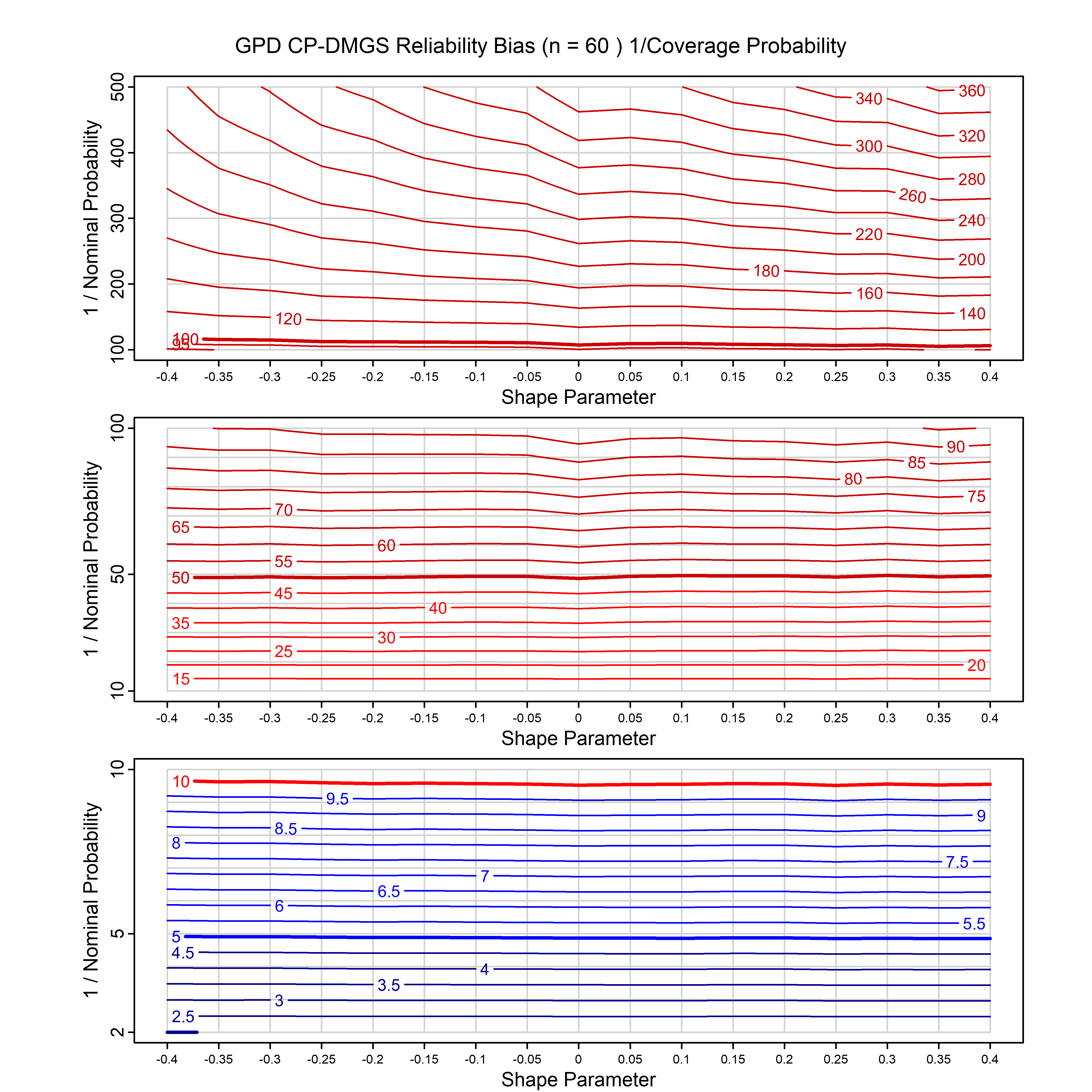
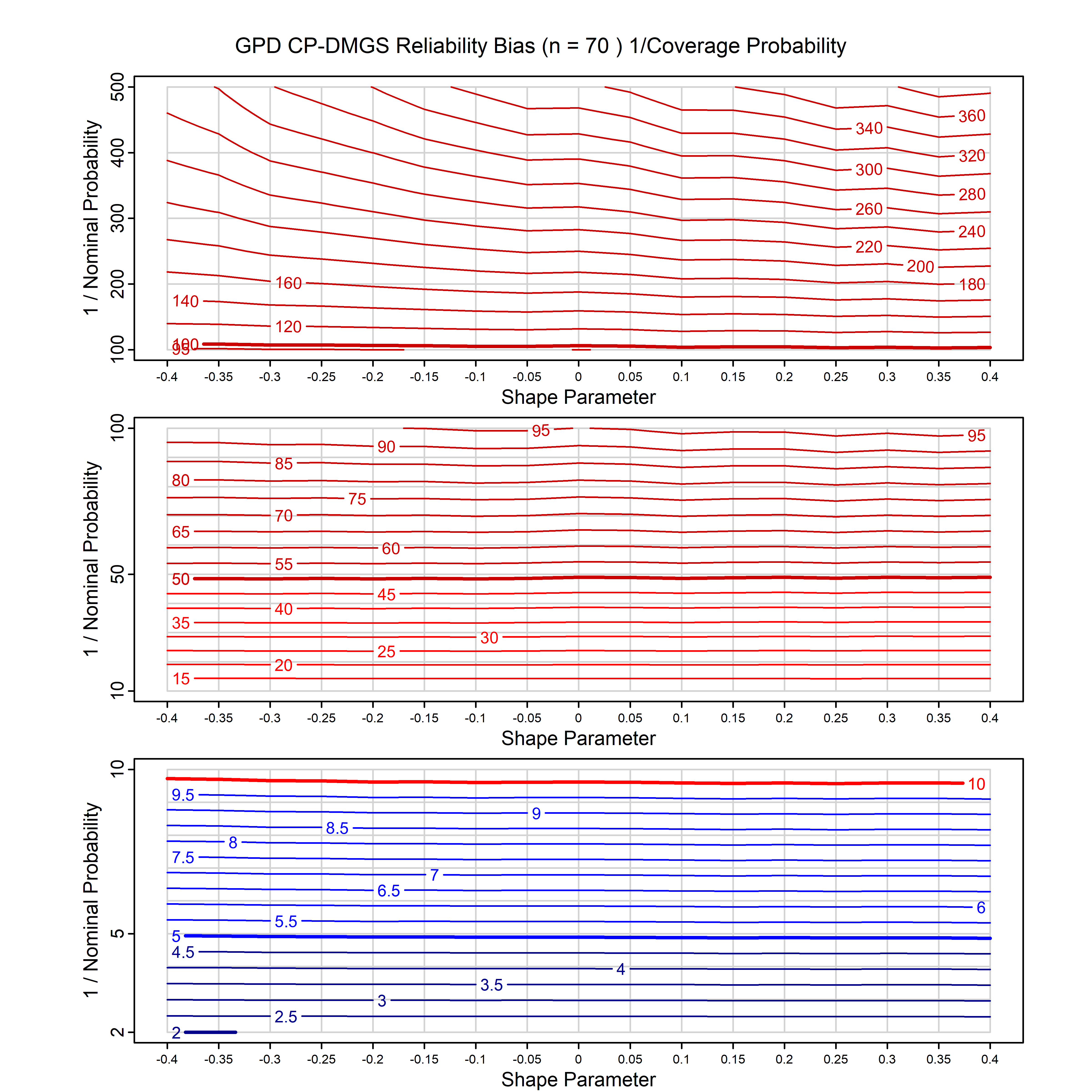
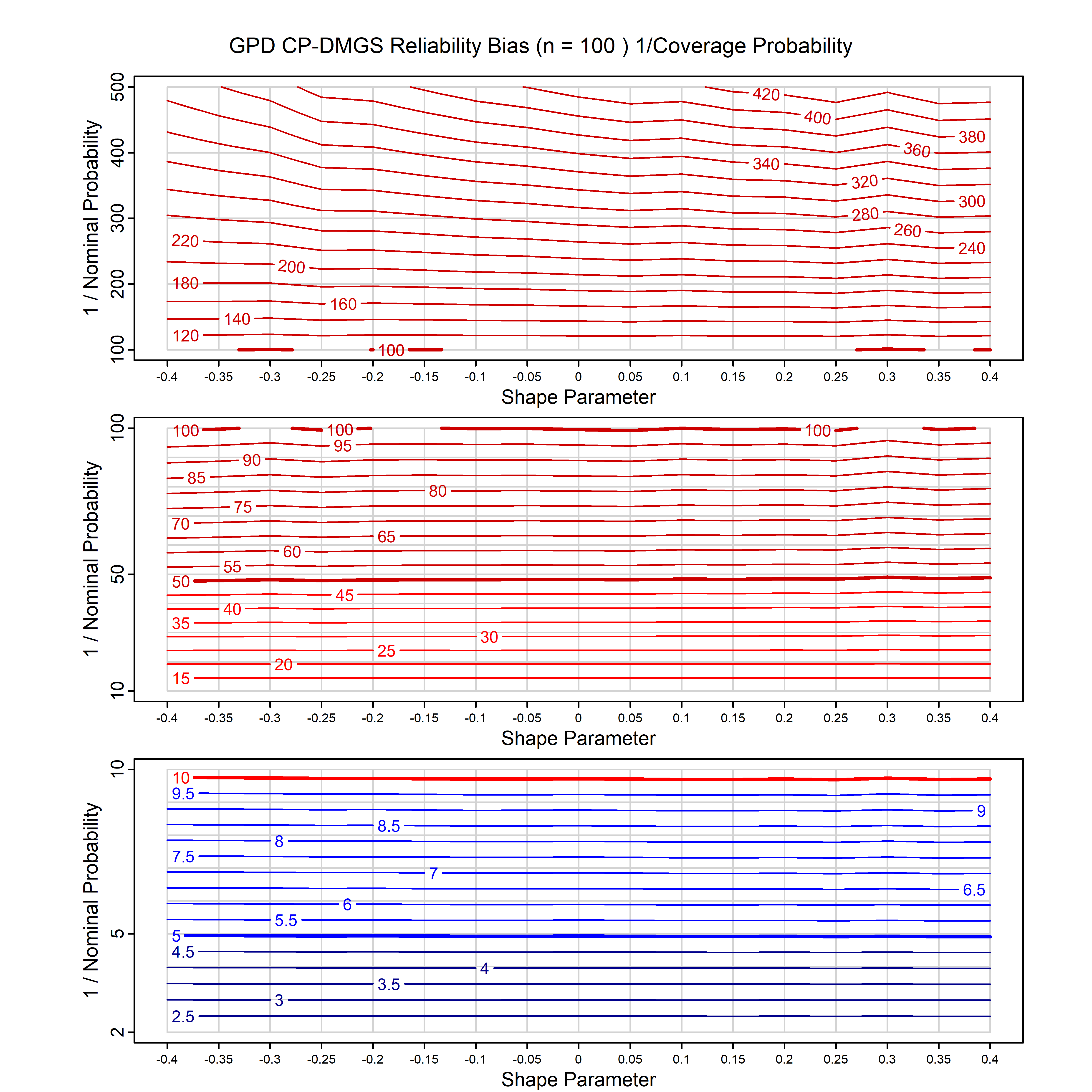
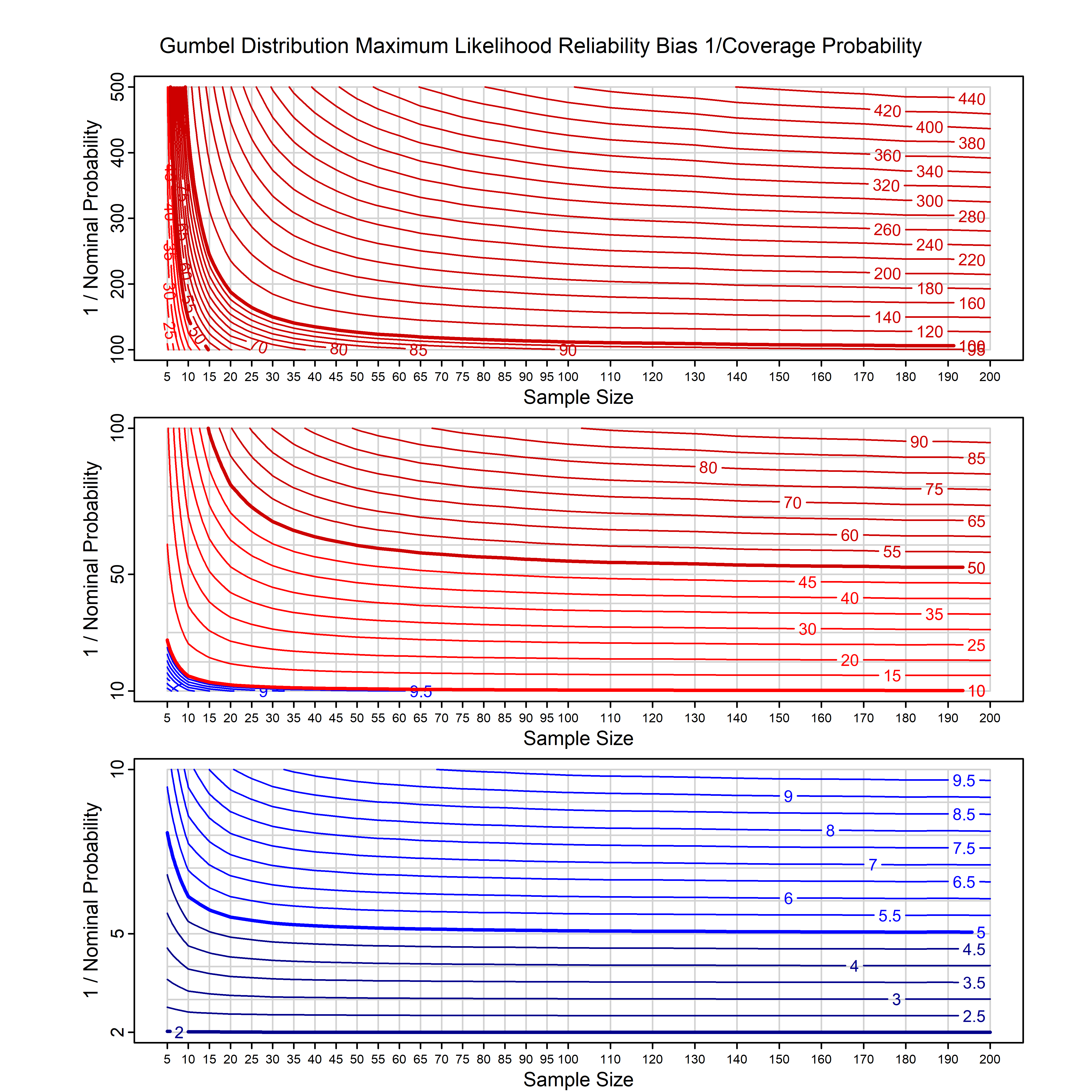
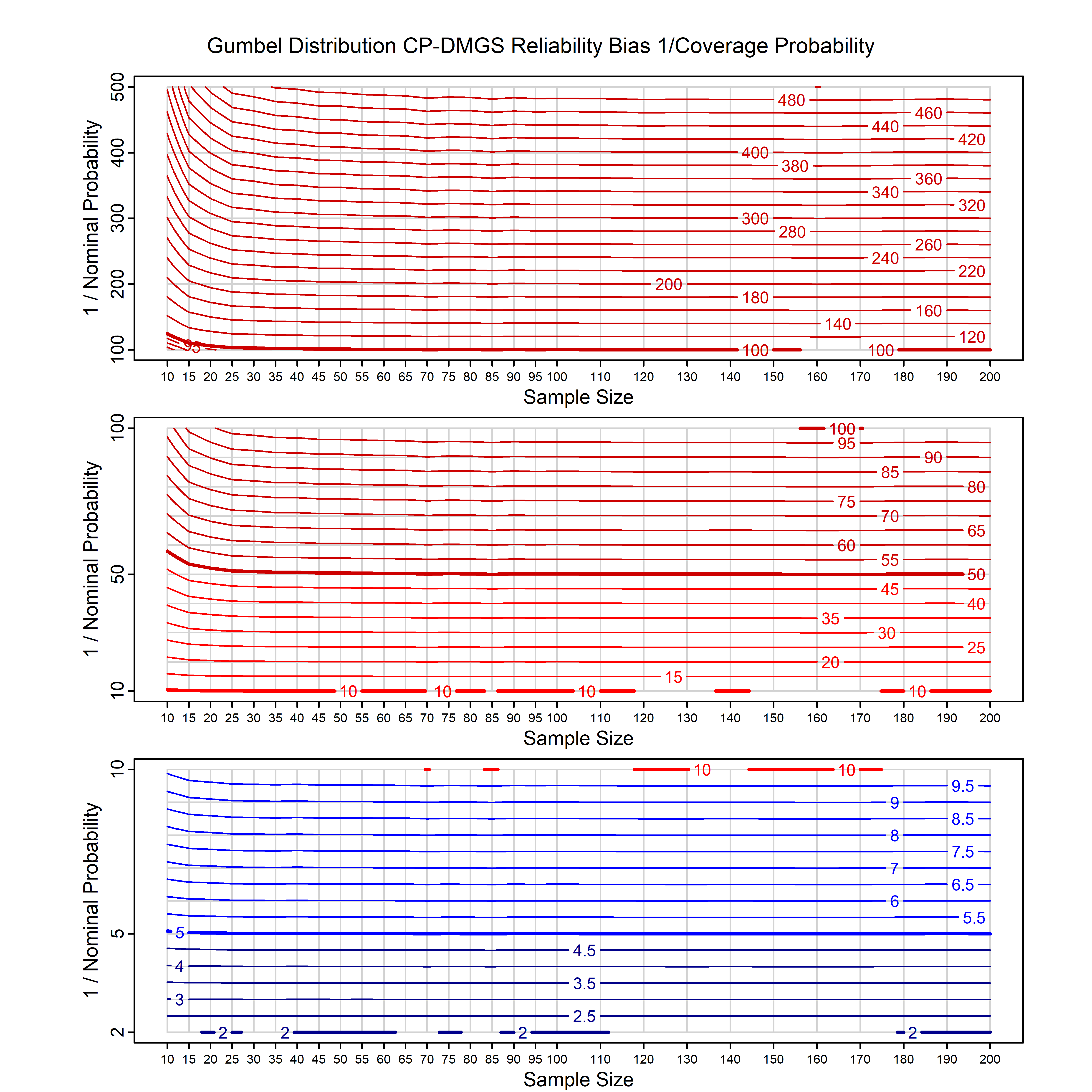
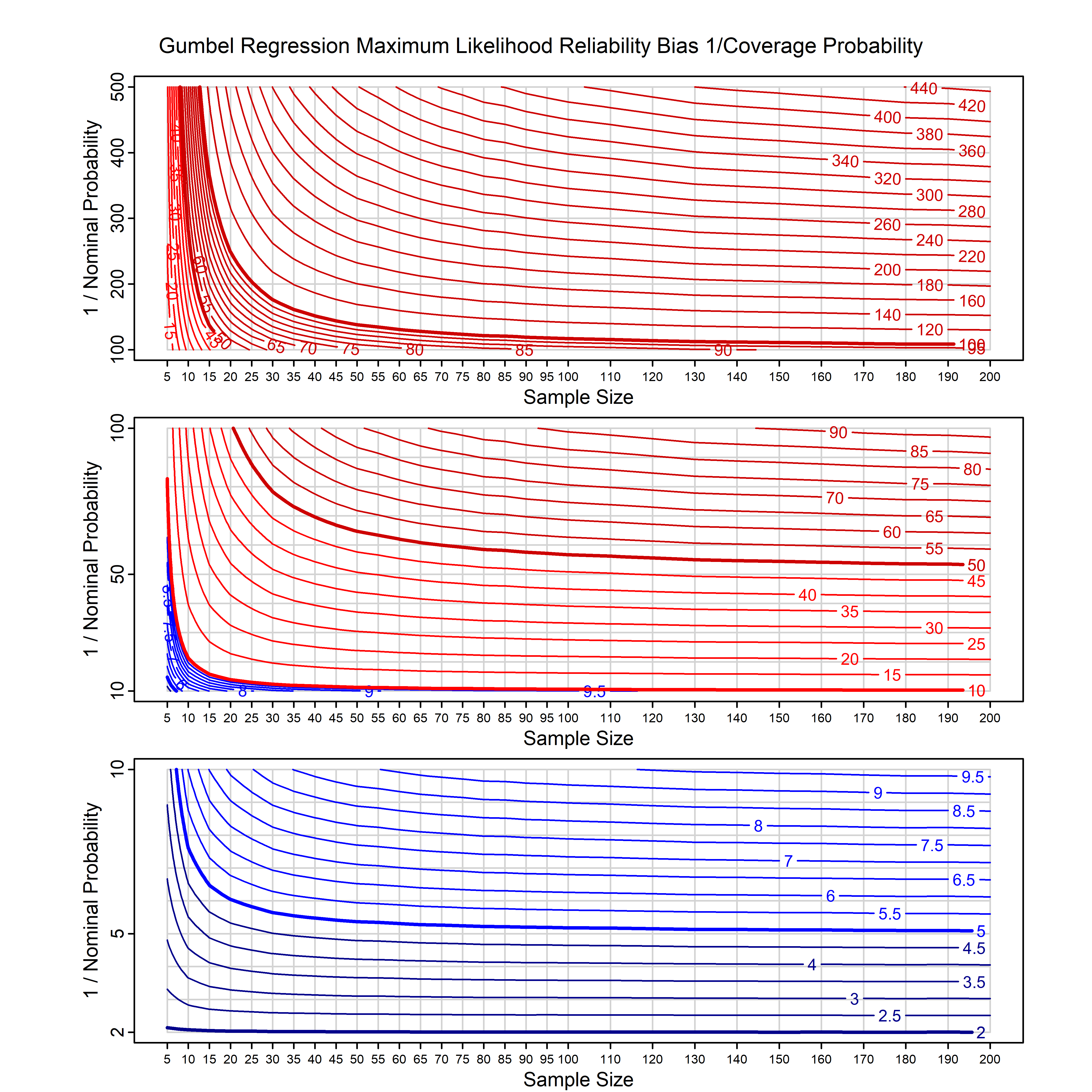
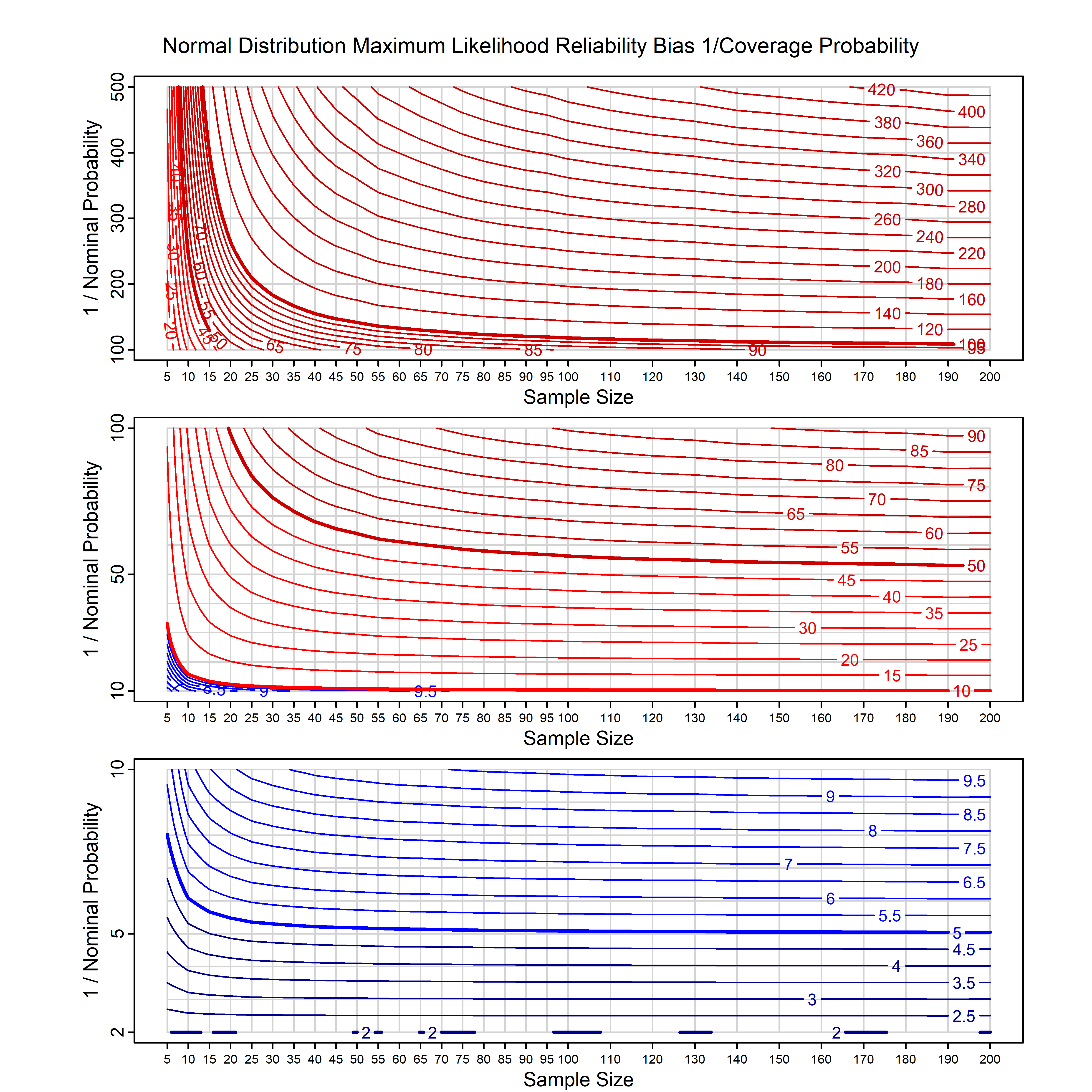
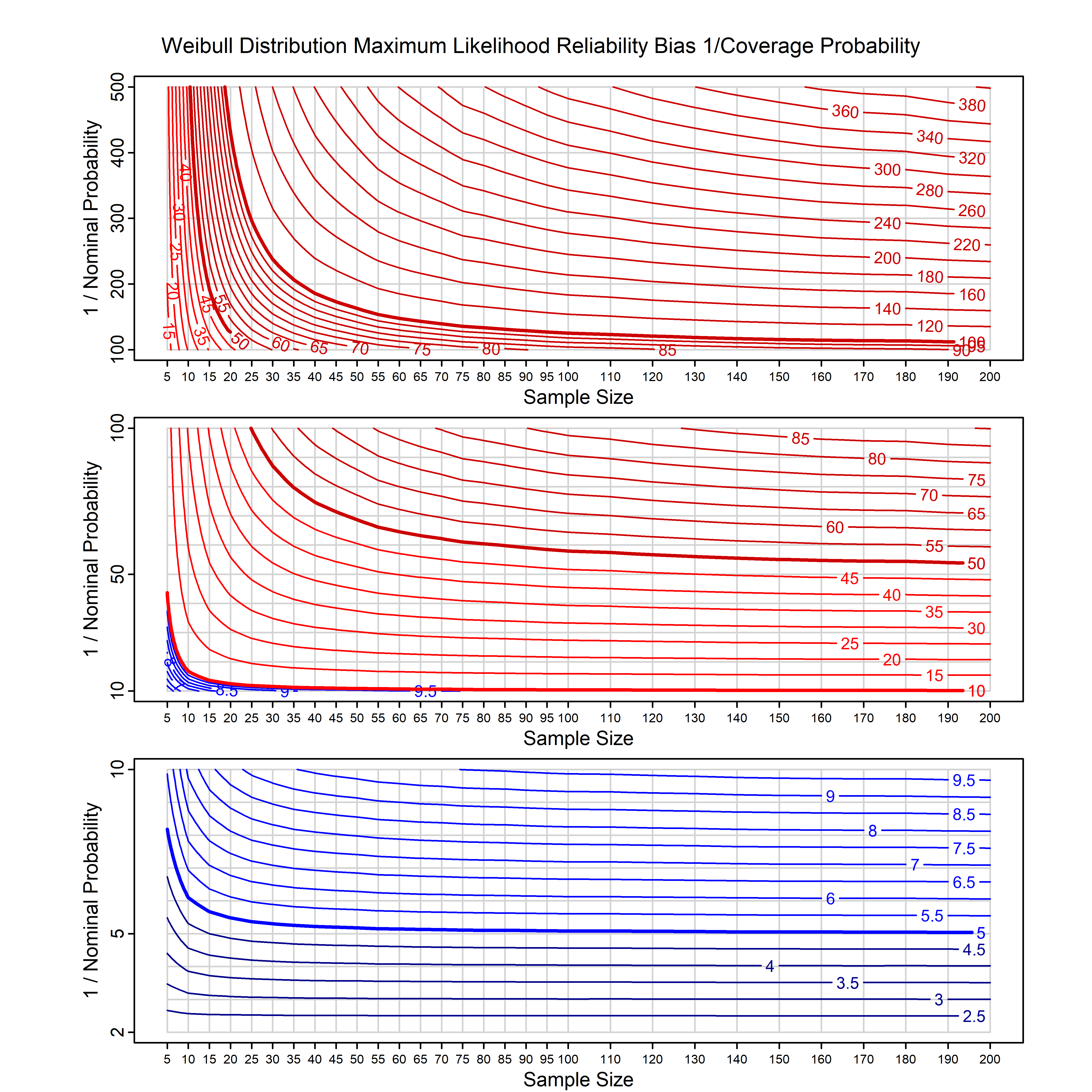
Standard methods for fitting distributions such as maximum likelihood, and other point estimate methods, underestimate predictive tail probabilities and so underestimate risk. For instance, with maximum likelihood prediction, the GEVD with one predictor and shape parameter of -0.3 fitted to 50 data points underestimates the 1 in 50 probability by a factor of 4. We call this a reliability bias.
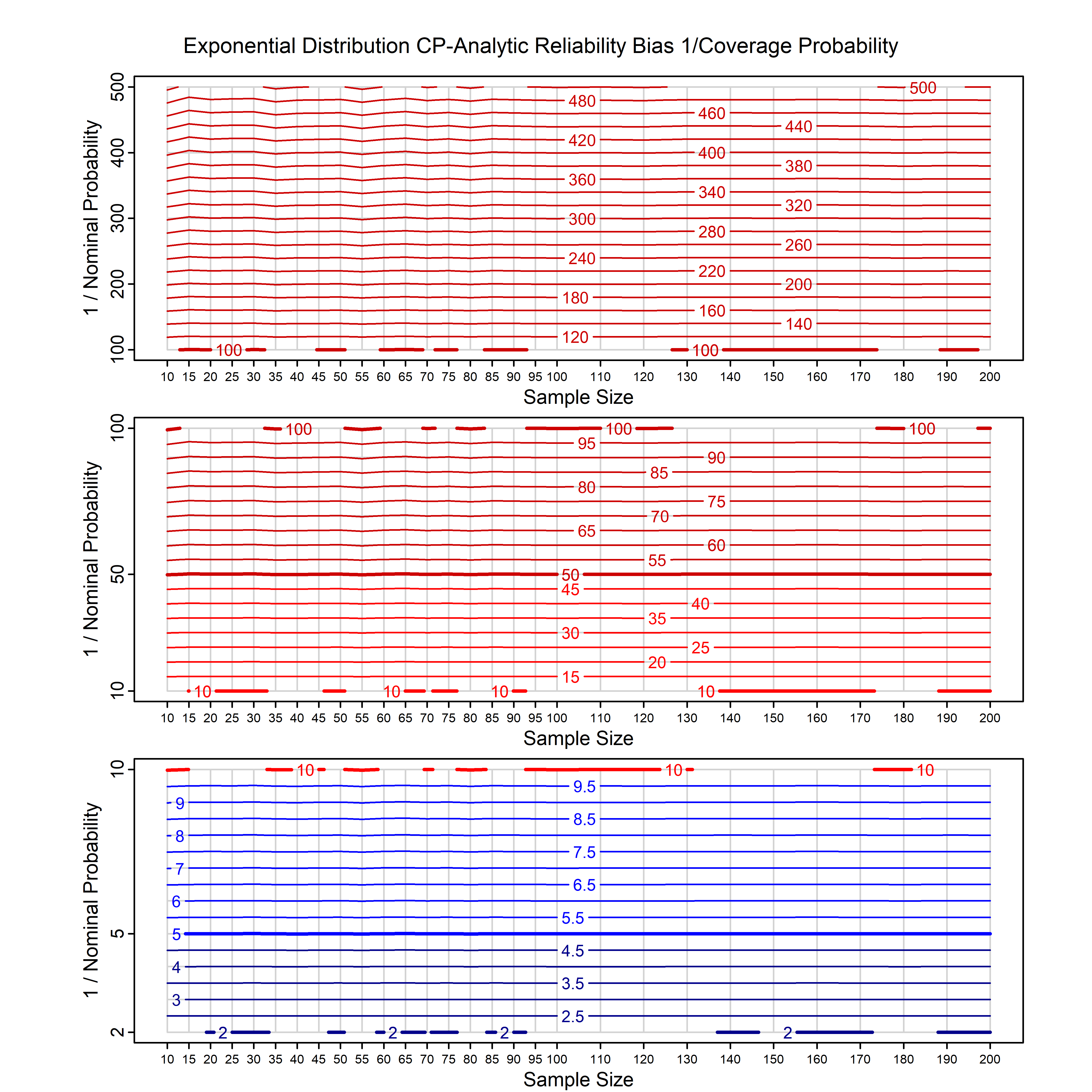
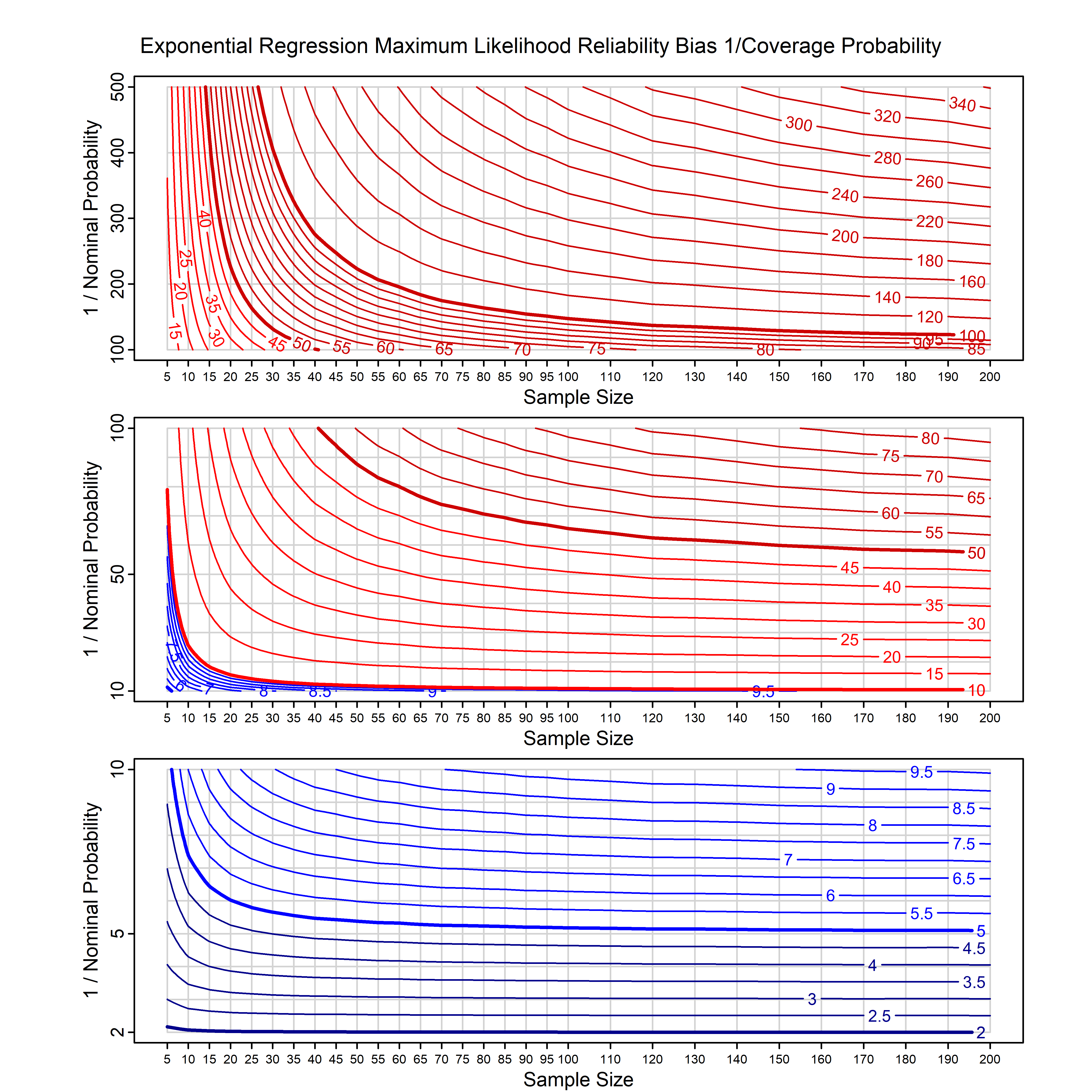
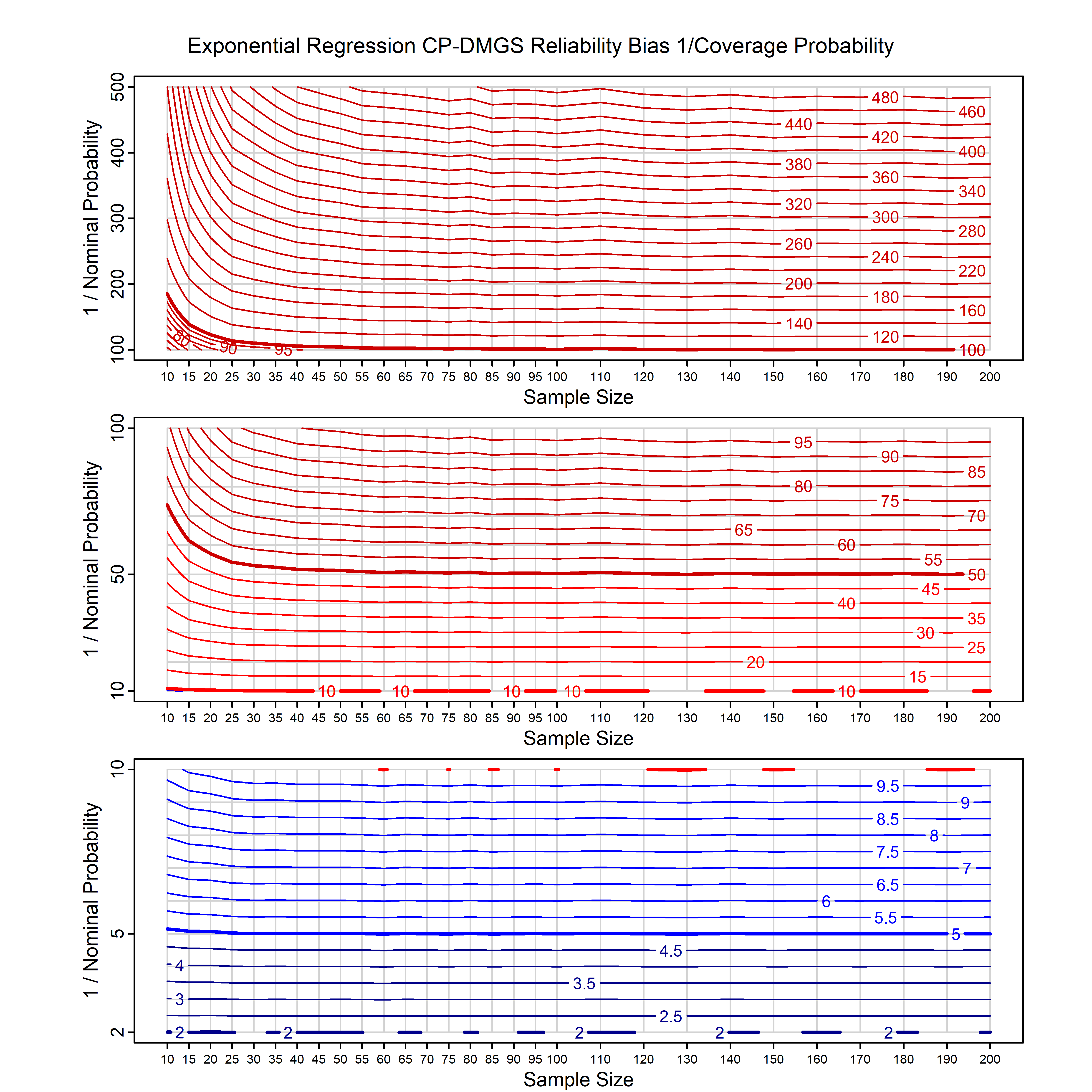
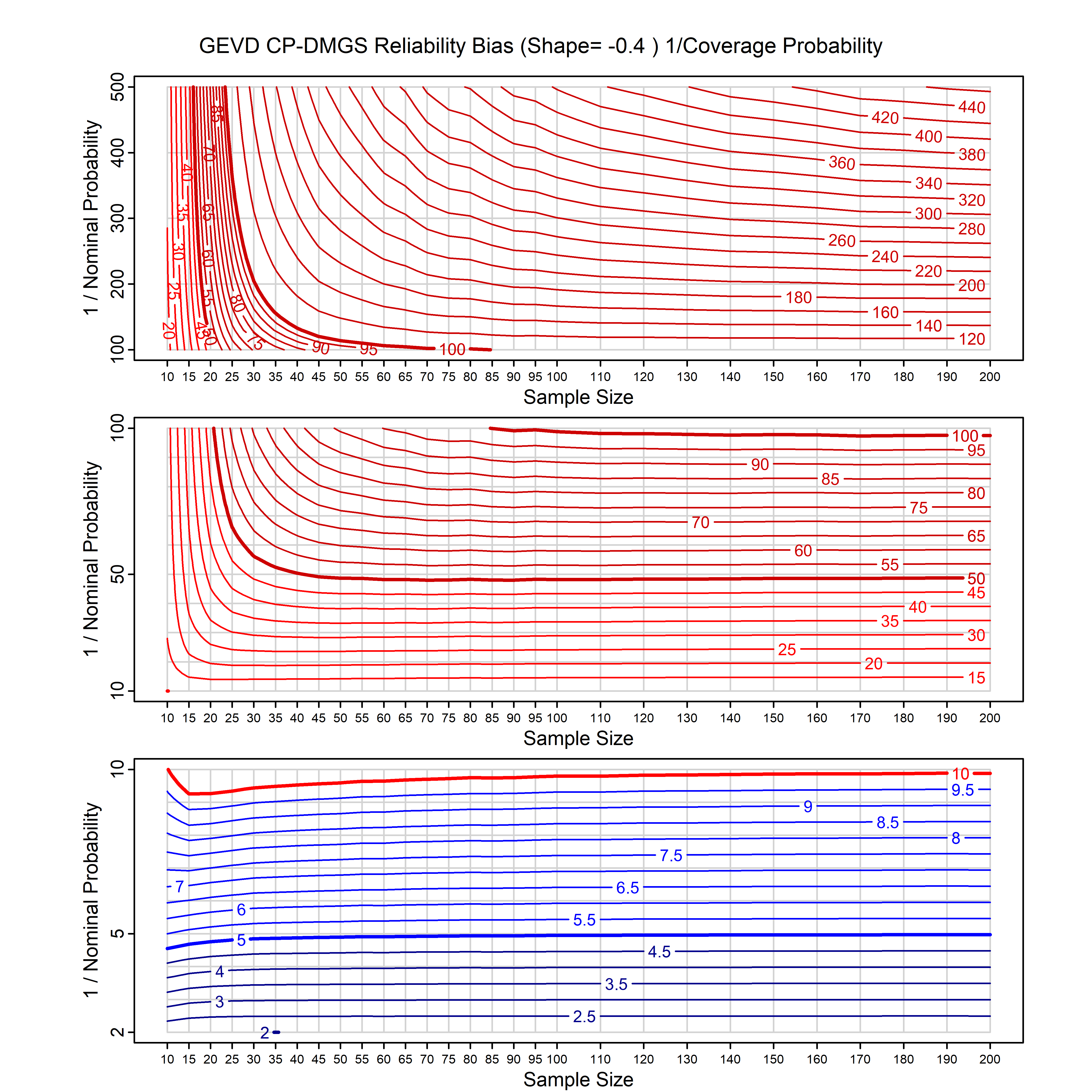
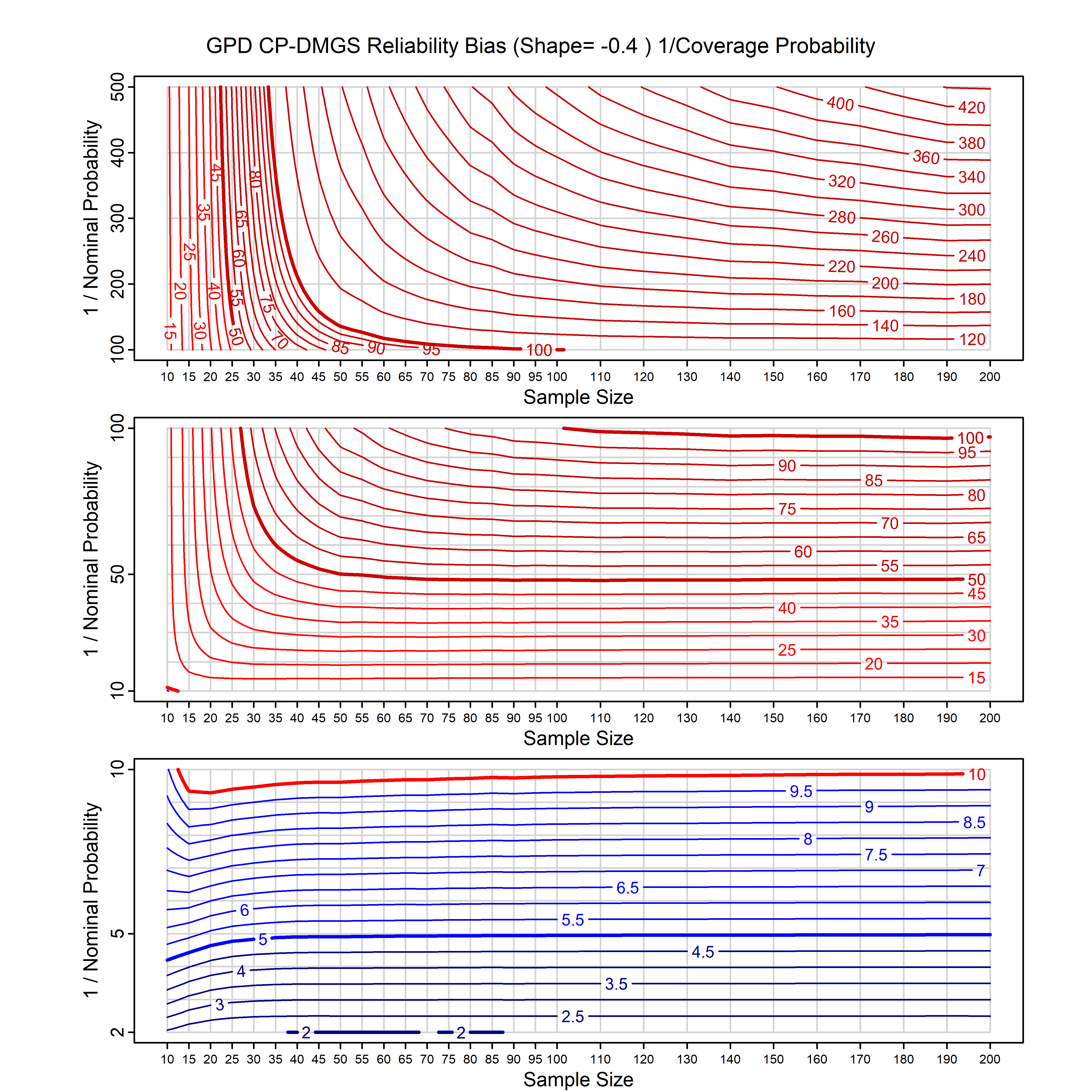
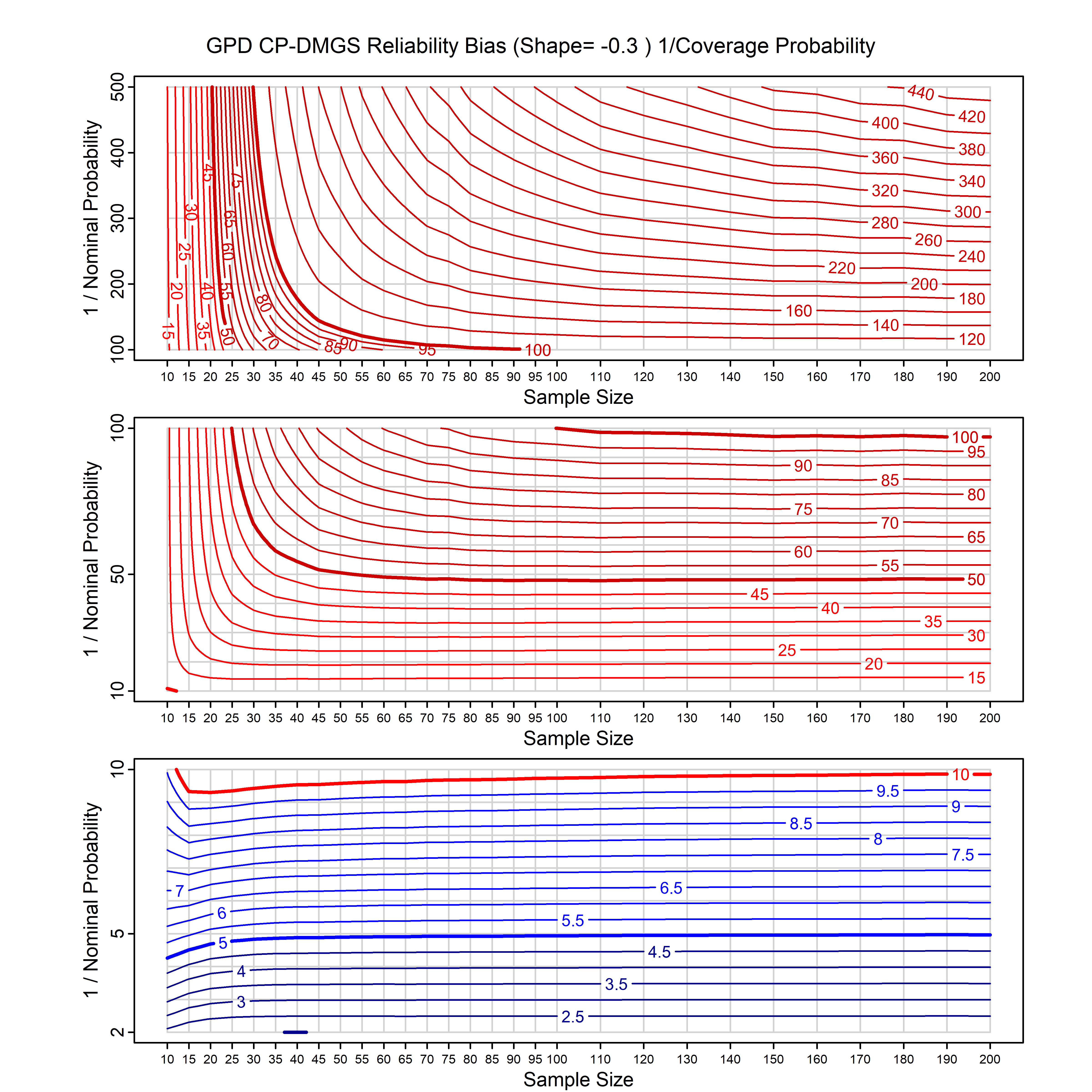
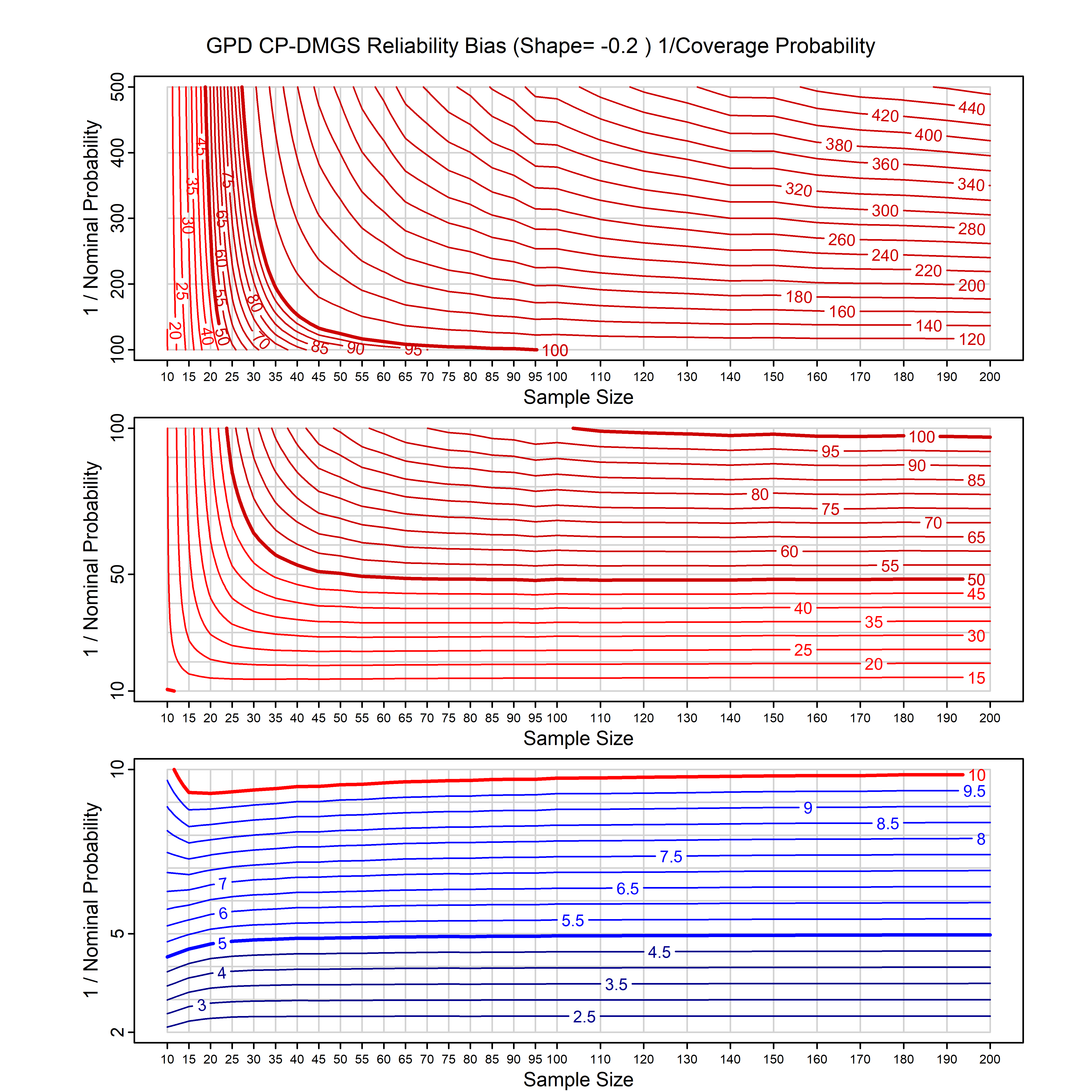
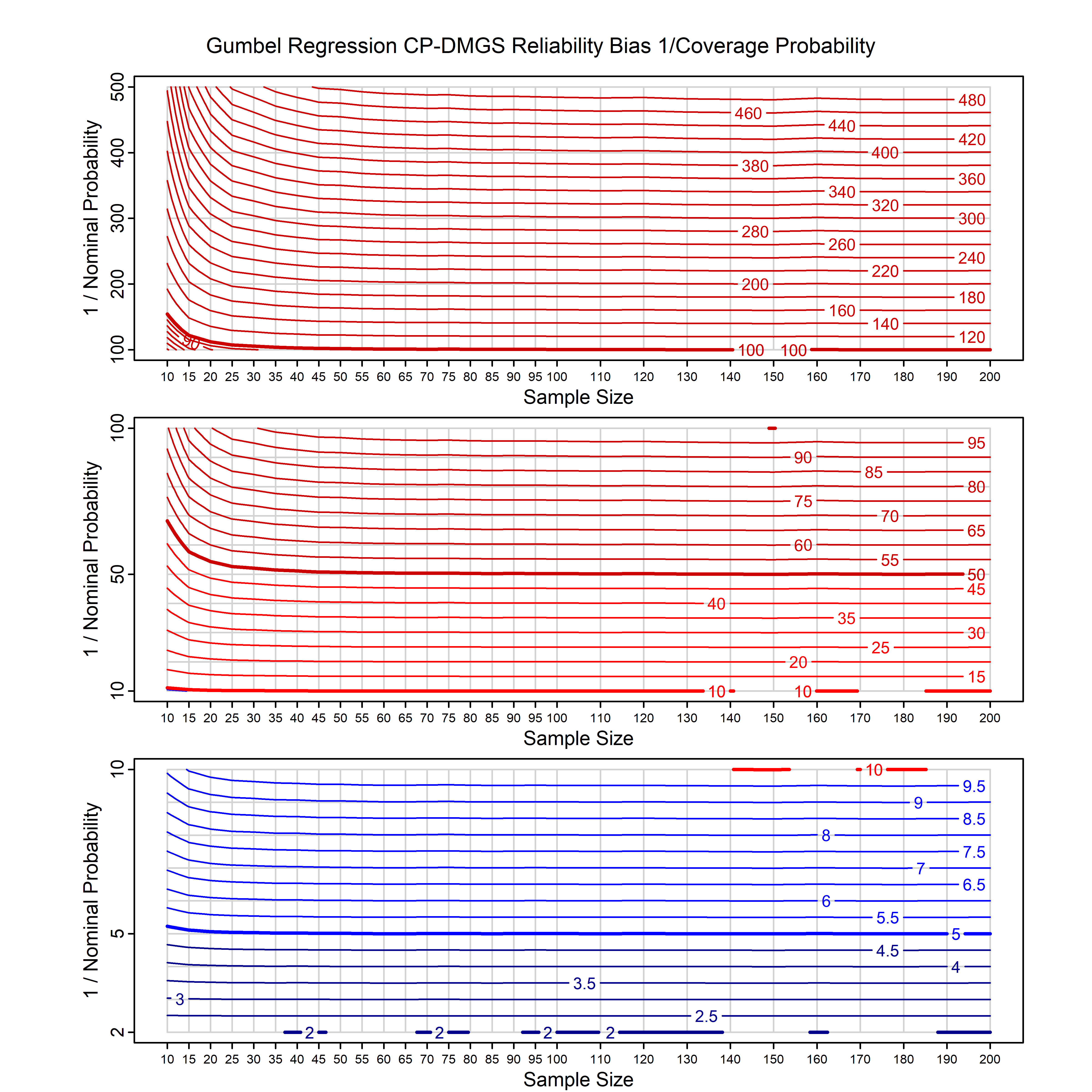
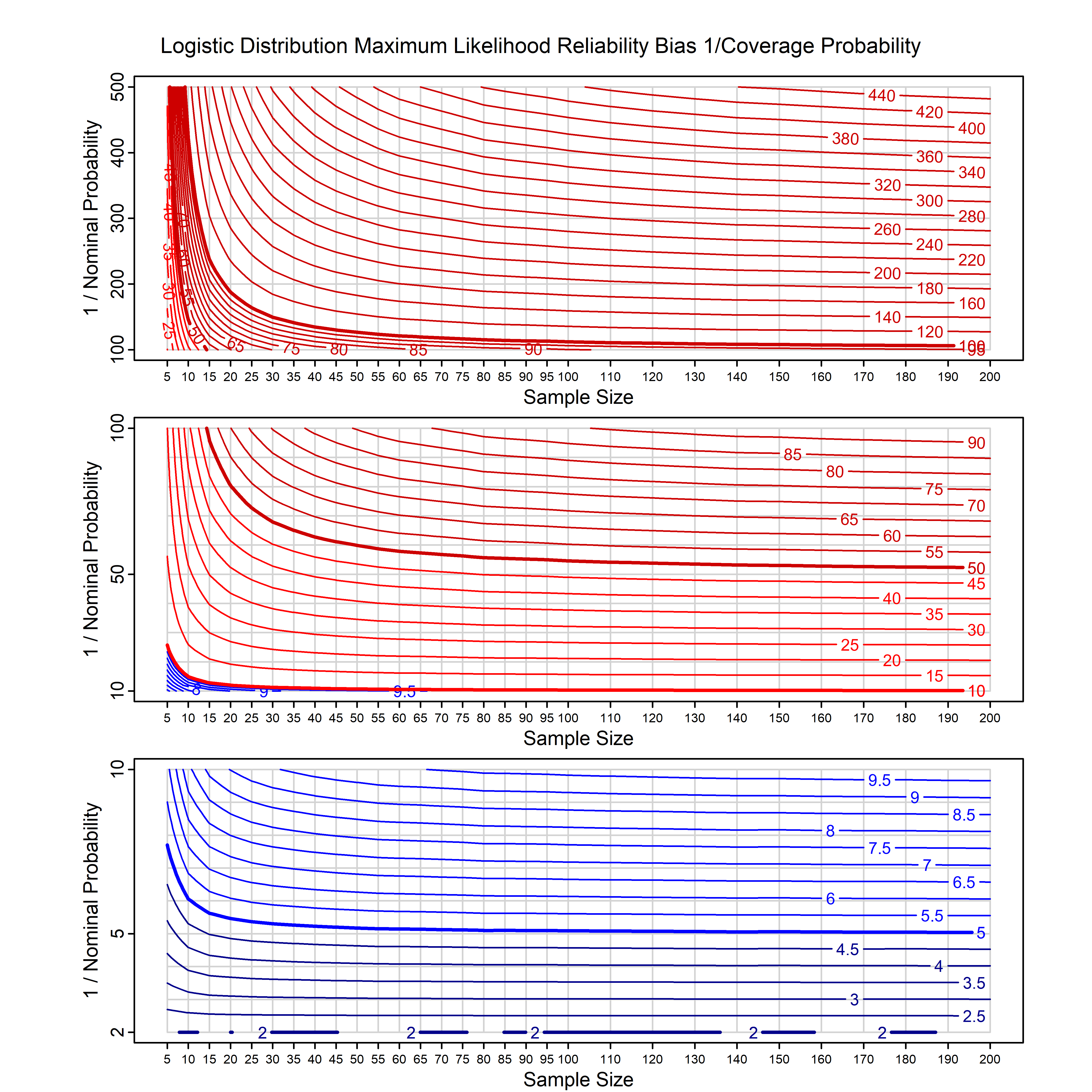
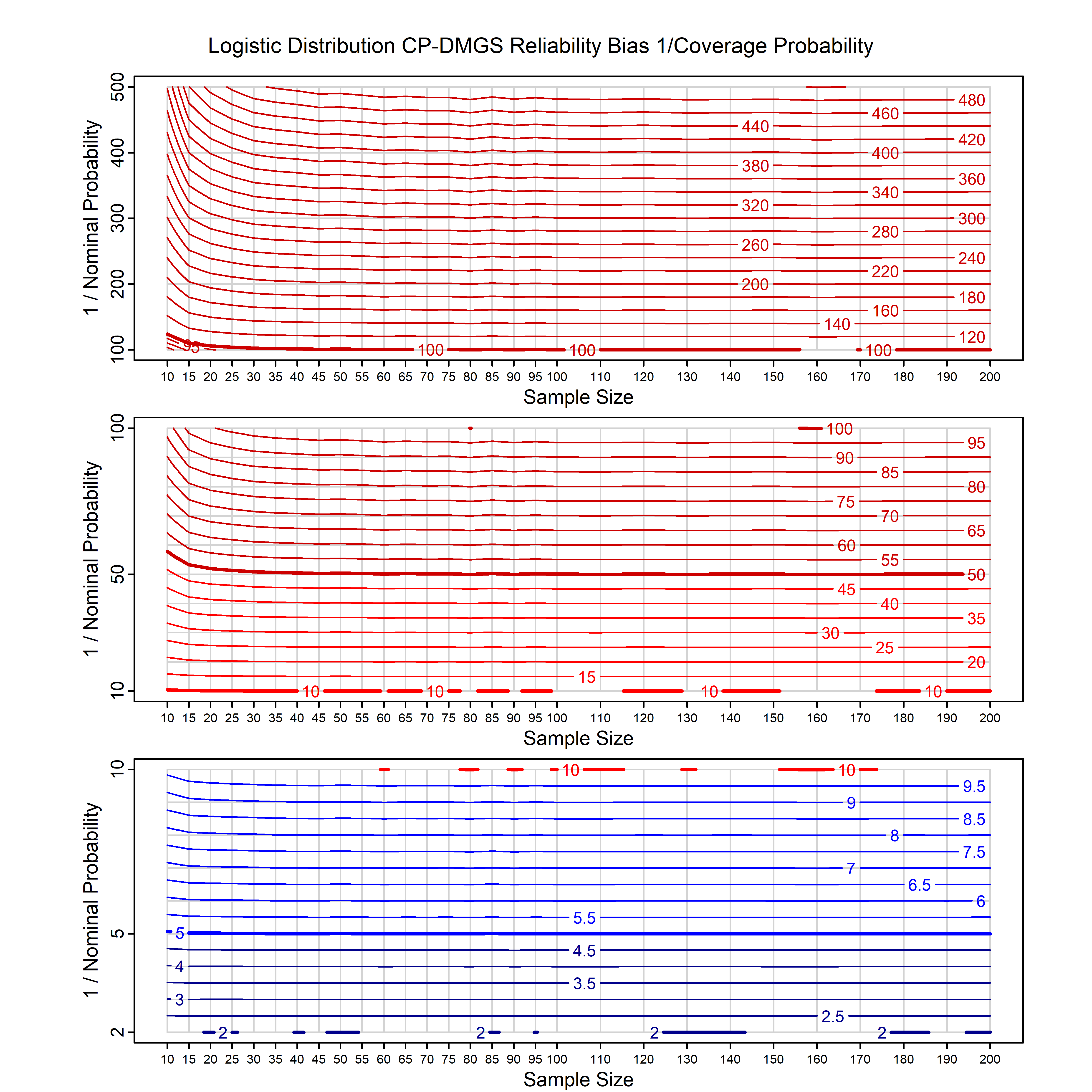
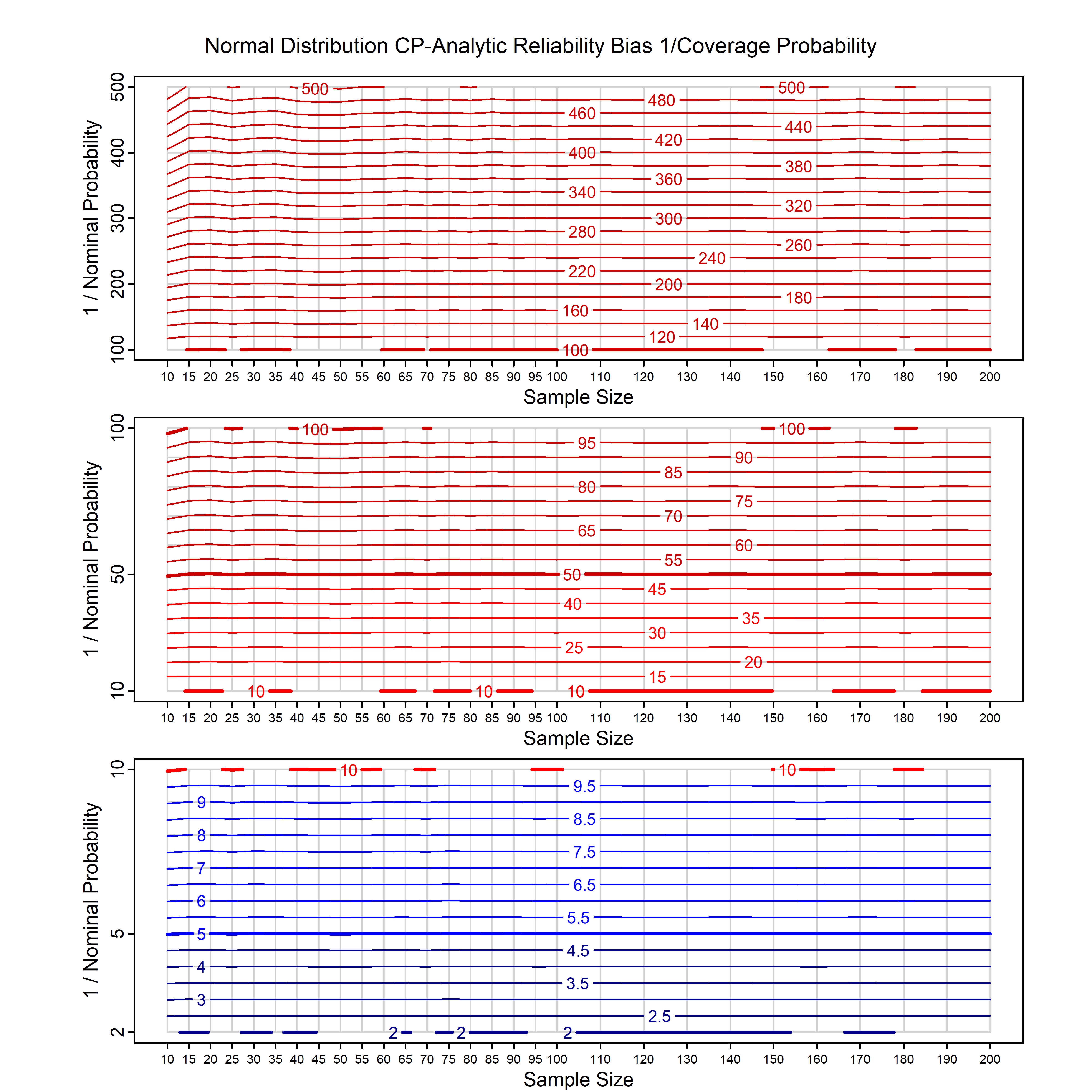
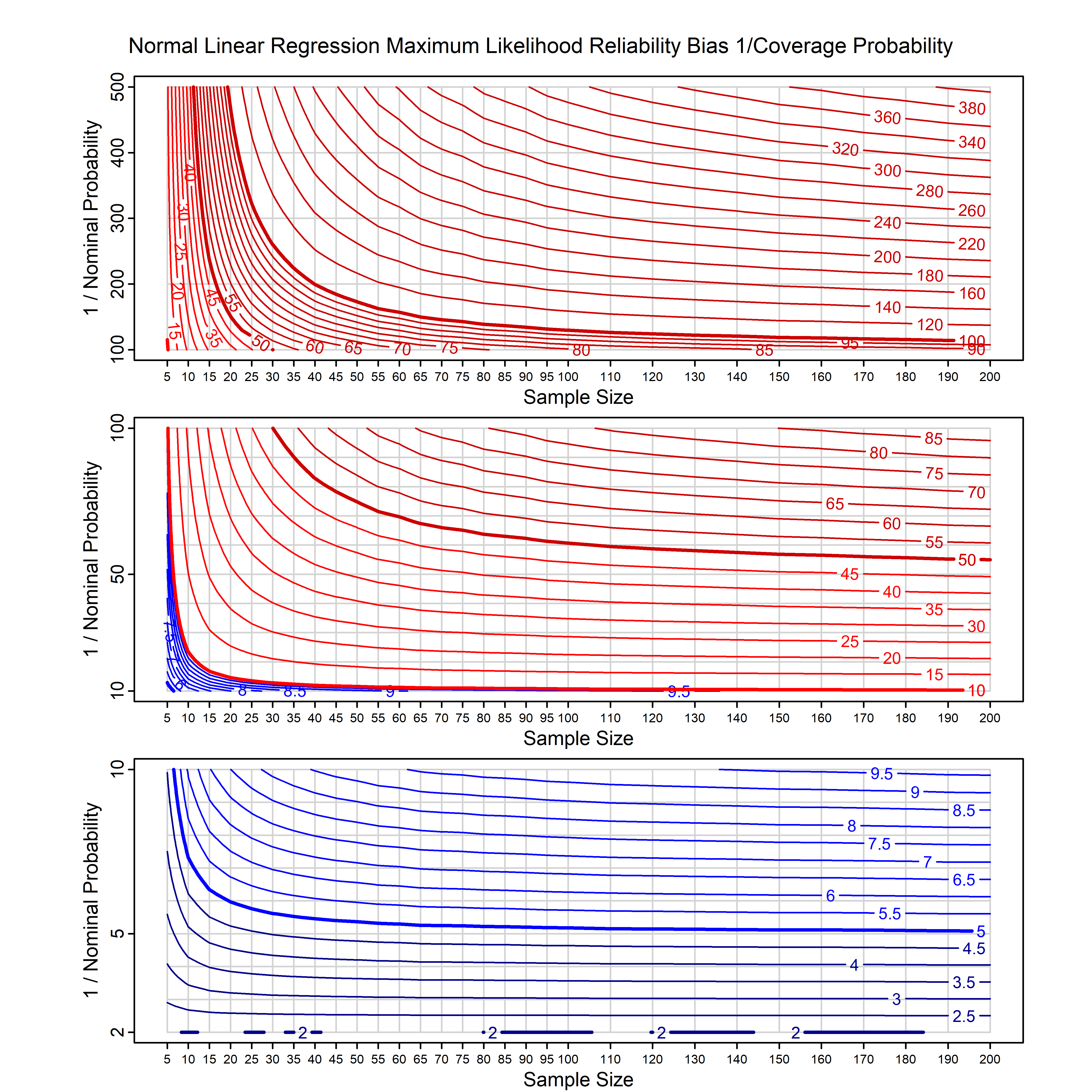
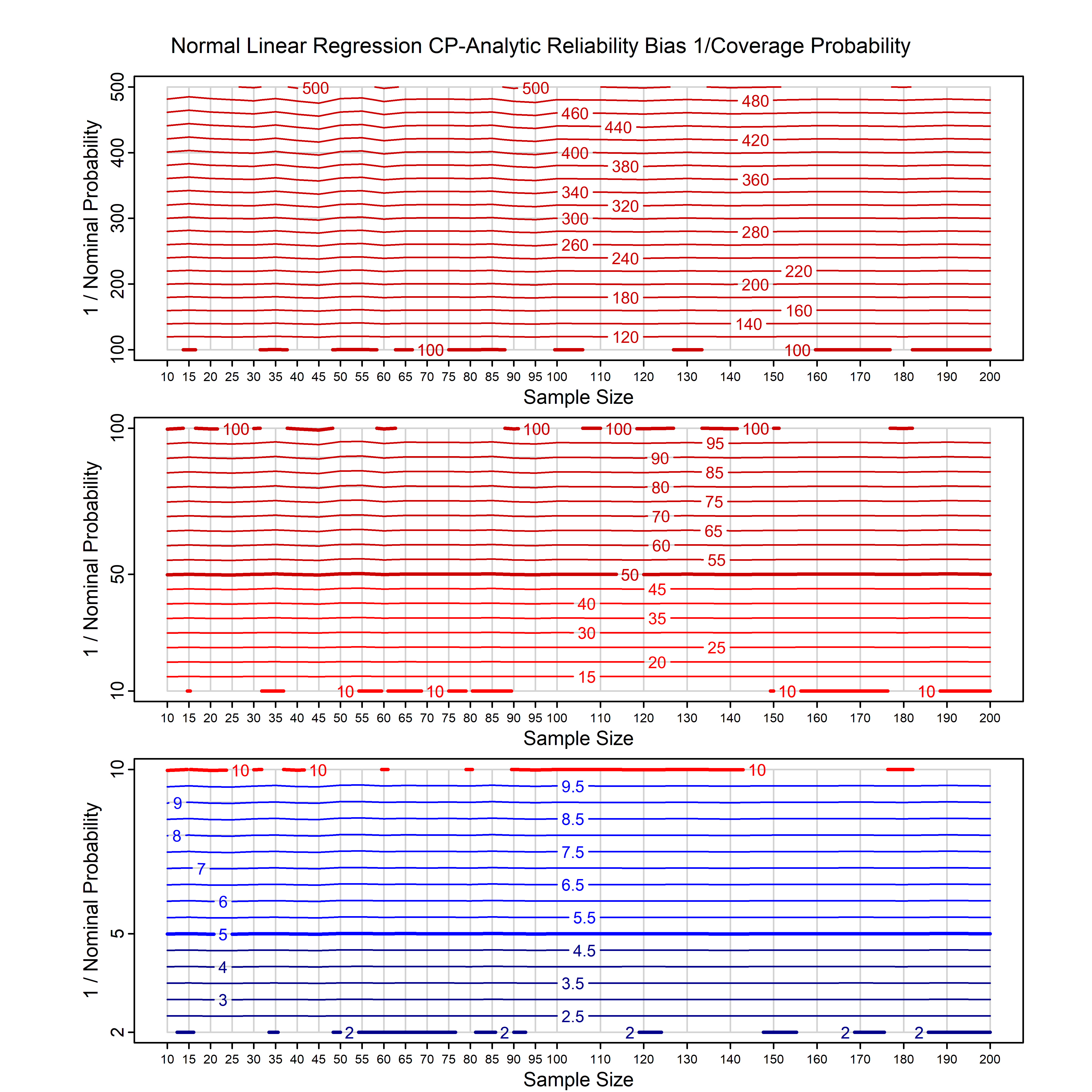
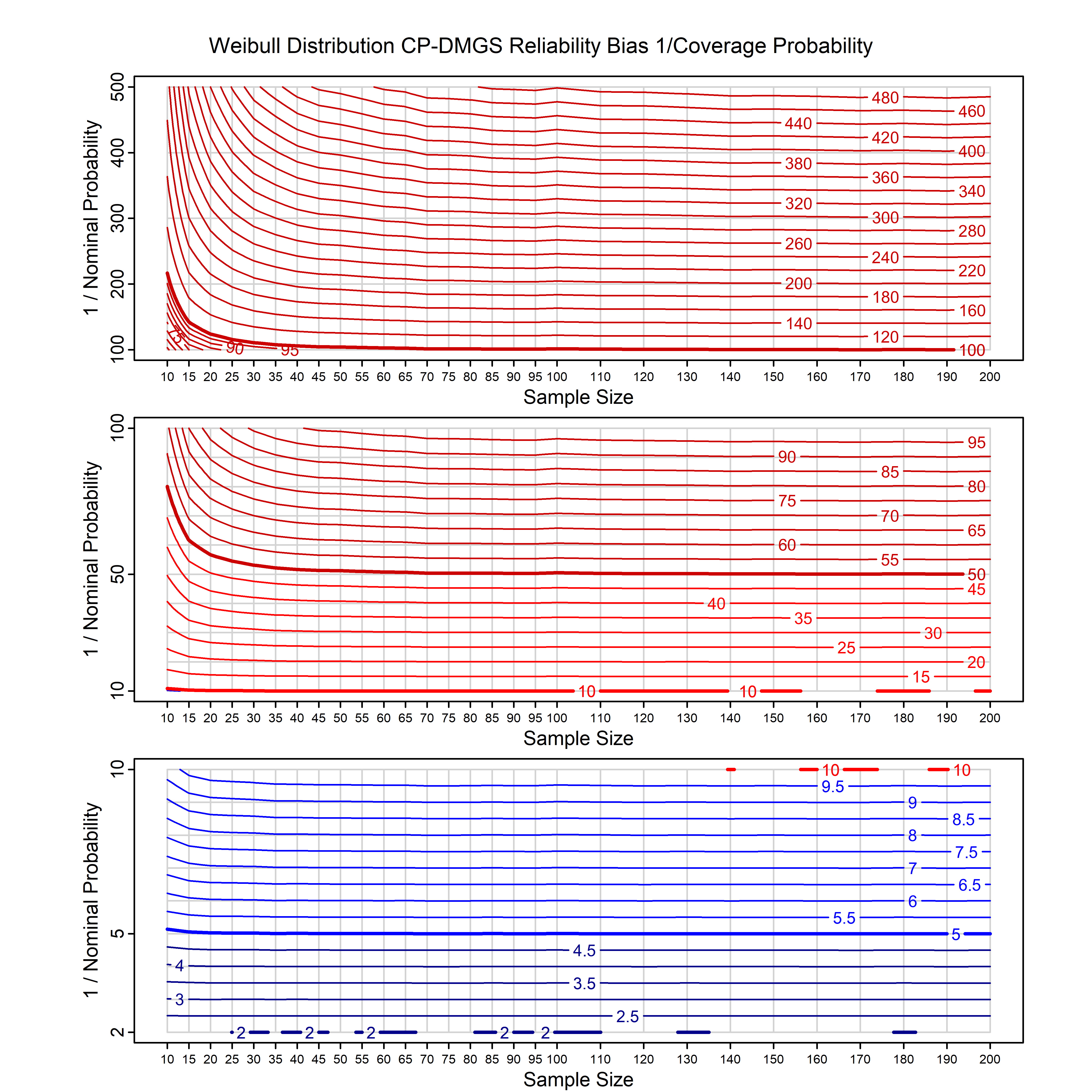
Calibrating prior prediction provides an objective way to reduce this reliability bias by including parameter uncertainty. It eliminates the bias completely in many cases, and reduces it greatly in others. The benefit of calibrating prior prediction, relative to maximum likelihood, is largest for small samples, models with more parameters, and in the tails.
The calibrating prior prediction method used for fitting distributions in fitdistcp uses objective Bayesian methods. The prior is chosen to maximize the reliability of the predictions,
i.e., to give predictive probabilities that are as close as possible to the frequencies of future outcomes.
The integration is performed analytically if possible, or using DMGS asymptotics otherwise.
Posterior sampling is also available as an option (but is slower).
For many distributions, charts are provided below that quantify the size of the maximum likelihood reliability bias, and the reduced bias from calibrating prior prediction.
R Models
This is a list of the models that are currently supported in the R version of fitdistcp, in alphabetical order.
This list is motivated by various climate and actuarial applications. Let us know if you have any suggestions for other models to include.
- The R command needs to be prefixed with one of
d,p,q,r,t H/Iindicates whether the model is homogenenous or inhomogeneous (i.e., is the transformation group sharply transitive or not).A/Dindicates whether the default integration method used infitdistcpis analytic or DMGS- In some cases, reliability bias charts are provided for maximum likelihood and calibrating prior predictions.
- For EVT models, the reliability bias charts are given as a function of the true shape parameter
| Model | R Command | H/I | A/D | Maxlik bias | CP bias |
|---|---|---|---|---|---|
| Cauchy | cauchy_cp | H | D | N/A | N/A |
| Cauchy with single predictor on the location | cauchy_p1_cp | H | D | N/A | N/A |
| Exponential | exp_cp | H | A | all parameters | all parameters |
| Exponential with single predictor on the rate | exp_p1_cp | H | D | all parameters | all parameters |
| Frechet with known location | frechet_k1_cp | H | D | all parameters | all parameters |
| Frechet with known location, and single predictor on the scale | frechet_k1p3_cp | H | D | N/A | N/A |
| Gamma | gamma_cp | I | D | N/A | N/A |
| Inverse gamma | invgamma_cp | I | D | N/A | N/A |
| Inverse Gaussian | invgauss_cp | I | D | N/A | N/A |
| Generalized normal with known shape | gnorm_cp | H | D | N/A | N/A |
| GEV | gev_cp | I | D | xi=-0.4, -0.3, -0.2, -0.1, 0, 0.1, 0.2, 0.3, 0.4 n=30, 40, 50, 60, 70, 80, 100, 120 | xi=-0.4, -0.3, -0.2, -0.1, 0, 0.1, 0.2, 0.3, 0.4 n=30, 40, 50, 60, 70, 80, 100, 120 |
| GEV with 1 predictor, on the location | gev_p1_cp | I | D | xi=-0.4, -0.3, -0.2, -0.1, 0, 0.1, 0.2, 0.3, 0.4 n=30, 40, 50, 60, 70, 80, 100, 120 | xi=-0.4, -0.3, -0.2, -0.1, 0, 0.1, 0.2, 0.3, 0.4 n=30, 40, 50, 60, 70, 80, 100, 120 |
| GEV with 1, 2 or 3 predictors on the location | gev_p1n_cp | I | D | N/A | N/A |
| GEV with 2 predictors, one each on the location and scale | gev_p12_cp | I | D | xi=-0.4, -0.3, -0.2, -0.1, 0, 0.1, 0.2, 0.3, 0.4 n=30, 40, 50, 60, 70, 80, 100, 120 | xi=-0.4, -0.3, -0.2, -0.1, 0, 0.1, 0.2, 0.3, 0.4 n=30, 40, 50, 60, 70, 80, 100, 120 |
| GEV with 3 predictors, one each on the location, scale and shape | gev_p123_cp | I | D | N/A | N/A |
| GEV with known shape | gev_k3_cp | H | D | N/A | N/A |
| GEV with known shape with a single predictor on the location | gev_k3p1_cp | H | D | N/A | N/A |
| GPD with known location | gpd_k1_cp | I | D | xi=-0.4, -0.3, -0.2, -0.1, 0, 0.1, 0.2 0.3 0.4 n=30, 40, 50, 60, 70, 80, 100, 120 | xi=-0.4, -0.3, -0.2, -0.1, 0, 0.1, 0.2 0.3 0.4 n=30, 40, 50, 60, 70, 80, 100, 120 |
| GPD with known location and shape | gpd_k13_cp | I | D | N/A | N/A |
| Gumbel | gumbel_cp | H | D | all parameters | all parameters |
| Gumbel with single predictor on the location | gumbel_cp | H | D | all parameters | all parameters |
| Half-normal | halfnorm_cp | H | D | N/A | N/A |
| Logistic | logis_cp | H | D | all parameters | all parameters |
| Logistic with single predictor on the location | logis_p1_cp | H | D | N/A | N/A |
| Log-normal | lnorm_cp | H | A | same as norm | same as norm |
| Log-normal with a single predictor on the log-mean | lnorm_p1_cp | H | A | same as norm_p1 | same as norm_p1 |
| Normal | norm_cp | H | A | all parameters | all parameters |
| Normal with 1 predictor, on the mean i.e., simple linear regression | norm_p1_cp | H | A | all parameters | all parameters |
| Normal with predictors on both parameters, i.e., heteroskedastic regression | norm_p12_cp | H | D | N/A | N/A |
| Pareto with known scale | pareto_k1_cp | H | A | same as exp | same as exp |
| Pareto with known scale and a single predictor on the shape parameter | pareto_p1k3_cp | H | D | same as exp_p1 | same as exp_p1 |
| t distribution with known degrees of freedom | lst_k3_cp | H | D | N/A | N/A |
| t distribution with known degrees of freedom with a single predictor on the location parameter | lst_p1k5_cp | H | D | N/A | N/A |
| Uniform | unif_cp | H | A | N/A | N/A |
| Weibull | weibull_cp | H | D | all parameters | all parameters |
| Weibull with single predictor on the scale | weibull_p2_cp | H | D | N/A | N/A |
R Examples
- Install
fitdistcpfrom CRAN usinginstall.packages("fitdistcp"). - Load
fitdistcpusinglibrary(fitdistcp).
R Example 1: Fitting a normal distribution and calculating the fitted probability density function
> x=rnorm(20)		# make some example training data
> y=seq(-5,5,0.01)	# define the points at which we wish to calculate the density
> d=dnorm_cp(x,y)	# this command calculates two sets of predictive densities for the normal, one based on maxlik,
			# and one that includes parameter uncertainty based on a calibrating prior
> print(d$ml_pdf)	# have a look at the maxlik densities
> print(d$cp_pdf)	# have a look at the densities that include parameter uncertainty, which will have fatter tails
R Example 2: Fitting a GEV distribution and calculating the fitted quantiles
> set.seed(1)
> x=rlogis(20)				# make some example training data
> p=seq(0.001,0.999,0.001)		# define the probabilities at which we wish to calculate the quantiles
> q=qgev_cp(x,p)			# this command calculates two sets of predictive quantiles for the GEV,
					# one based on maxlik, and one that includes parameter uncertainty based on a calibrating prior
> q$ml_params 				# have a look at the maxlik parameters
> plot(q$ml_quantiles,p)		# plot the maxlik quantiles
> points(q$cp_quantiles,p,col="red")	# overplot the quantiles that include parameter uncertainty, which will have fatter tails
R Example 3: Fitting a GPD and calculating the fitted cumulative distribution function
> set.seed(1)
> x=rlnorm(20,sdlog=2)		# make some example training data (all positive values)
> y=seq(0.1,5,0.1)		# define the points at which we wish to calculate the probabilities
> p=pgpd_k1_cp(x,y)		# this command calculates two sets of predictive probabilities for the GPD (with known location parameter, hence k1),
				# one based on maxlik, and one that includes parameter uncertainty based on a calibrating prior
> plot(y,p$ml_cdf)		# have a look at the maxlik probabilities
> point(y,p$cp_pdf,col="red")	# have a look at the probabilities that include parameter uncertainty,
				# which will have fatter tails
R Example 4: Fitting a Gumbel distribution and generating random numbers
> x=rnorm(10)					# make some example training data
> r=rgumbel_cp(10000,x)				# this command calculates two sets of 10,000 predictive random numbers,
						# based on maxlik, and then with parameter uncertainty based on a calibrating prior
> plot(density(r$ml_deviates))			# plot the density of the maxlik random numbers
> lines(density(r$cp_deviates),col="red")	# overplot the density of the random numbers including parameter uncertainty,
						# which will have fatter tails
R Example 5: Generating posterior samples from a Weibull distribution
> x=rlnorm(20)						# make some example training data (all positive values)
> t=tweibull_cp(1000,x)$theta_samples			# this command generates 1000 posterior samples
R Example 6: Fitting a GEV distribution with a predictor on the location parameter
> set.seed(1)
> n=30
> t=0.1*c(1:n)/n			# make an example predictor
> x=t+rlogis(n)				# make training data based on the predictor
> t0=t[n]				# set the value of the predictor at which to make the prediction
> p=seq(0.001,0.999,0.001)		# specify the probabilities at which to generate quantiles
> q=qgev_p1_cp(x,t,t0=t0,n0=NA,p) 	# specify either t0, or n0, and make the other one NA
R Example 7: Fitting a GEV distribution with predictors on location and scale parameters
> set.seed(1)
> n=50
> t1=0.1*c(1:n)/n					# make the first predictor
> t2=0.2*c(1:n)/n					# make the second predictor
> x=(t1+rlogis(n))*t2					# make training data based on the predictors
> n0=n							# set the values of the predictors at which to make the prediction
> p=seq(0.001,0.999,0.001)
> q=qgev_p12_cp(x,t1,t2,t01=NA,t02=NA,n01=n0,n02=n0,p)	# specify either t0, or n0, and make the other one NA
Detailed R Examples by model
The short examples are also given in the help pages accessible from within R (for example, in R, type >?norm_cp).
| Model | Short example | Long example |
|---|---|---|
| Cauchy | R code | R code |
| Cauchy with single predictor on the location | R code | R code |
| Exponential | R code | R code |
| Exponential with single predictor on the rate | R code | R code |
| Frechet with known location | R code | R code |
| Frechet with known location, and single predictor on the scale | R code | R code |
| Gamma | R code | R code |
| Inverse gamma | R code | R code |
| Inverse Gaussian | R code | R code |
| Generalized normal with known shape | R code | R code |
| GEV | R code | R code |
| GEV with 1 predictor, on the location | R code | R code |
| GEV with 2 predictors, one each on the location and scale | R code | R code |
| GEV with 3 predictors, one each on the location, scale and shape | R code | R code |
| GEV with known shape | R code | R code |
| GEV with known shape with a single predictor on the location | R code | R code |
| GPD with known location | R code | R code |
| GPD with known location and shape | R code | R code |
| Gumbel | R code | R code |
| Gumbel with single predictor on the location | R code | R code |
| Half-normal | R code | R code |
| Logistic | R code | R code |
| Logistic with single predictor on the location | R code | R code |
| Log-normal | R code | R code |
| Log-normal with a single predictor on the log-mean | R code | R code |
| Normal | R code | R code |
| Normal with 1 predictor, on the mean i.e., simple linear regression | R code | R code |
| Pareto with known scale | R code | R code |
| Pareto with known scale and a single predictor on the shape parameter | R code | R code |
| t distribution with known degrees of freedom | R code | R code |
| t distribution with known degrees of freedom with a single predictor on the location parameter | R code | R code |
| Uniform | R code | R code |
| Weibull | R code | R code |
| Weibull with single predictor on the scale | R code | R code |
Theory
The theory behind calibrating prior prediction is discussed in detail in the citation given below. Here are some brief notes.- The goal is to make predictions that are as reliable as possible. Reliable means that events that are predicted to occur with a probability of 1% will indeed occur 1% of the time. Predictions from point estimate methods such as maximum likelihood are not reliable, and underestimate the tails.
- The predictions with parameter uncertainty are generated using the Bayesian prediction equation.
- Bayesian prediction requires a prior. For homogeneous models (i.e., models with sharply transitive transformation groups), we use the right Haar prior, which gives predictions that are in principle exactly reliable (if the model assumptions are correct, and depending on the integration scheme used). This applies to our Cauchy, exponential, Frechet, generalized normal, GEV with known shape, Gumbel, halfnormal, logistic, log-normal, normal, Pareto, t and Weibull models. It also applies to all these models with predictors.
- For inhomogeneous models (i.e., models without sharply transitive transformation groups) there is no solution that gives exact reliability, so we use simple priors that we have found will give close to exact reliability. They are in all cases more reliable than maxlik, but may not be very reliable for small sample size (e.g., n<50). This applies to GEV, GPD, gamma, inverse gamma and inverse Gaussian, and these models with predictors. We have even better priors for all these models in the pipeline.
- Simulations can be used to test whether a certain prior gives reliable predictions, as a function of the true parameters.
Simulation results are given in the reference paper cited below, and can be reproduced using the command
reltest. - Where possible, we integrate the Bayesian prediction equation analytically. This applies to the exponential, normal, log-normal, uniform and Pareto.
- Otherwise, by default we integrate the Bayesian prediction equation using the DMGS asymptotic expansion, which works well except for very small samples (n<10) (although even for very small sample sizes calibrating priors with DMGS still give more reliable predictions than maximum likelihood). DMGS is very fast, especially for quantiles (~1000x faster than MCMC).
- DMGS requires the calculation of various derivatives. Where possible, we use analytic expressions. Otherwise, we use simple numerical derivatives.
- There is also an option to integrate using posterior sampling, which then uses Paul Northrop's
rustlibrary (ratio of uniforms with transformation). Posterior sampling is slower than DMGS for the same level of accuracy (and for quantiles, much slower), but is ultimately more accurate if enough posterior samples are used.
Other Functionality
There are various other outputs, various additional options, and various related software tools are included in the package.- All calculations return the maxlik parameter estimates
- All calculations with the
q***_cp(ppfin Python) routines calculate the AIC and standard errors. AIC is presented as MAIC, which is -0.5 times the standard AIC, for better comparison with log scores, and so that higher is better. - Optionally, WAIC and out-of-sample log-score can be calculated too (although oos log-score can't be calculated for EVT routines, for mathematical reasons)
- Model selection can be illustrated using the
ms_flat_1tail, ms_flat_2tail, ms_predictors_1tailandms_predictors_2tailroutines.
>?gev_cp).
Running R from Python
The R package currently has more options than the Python package. For any missing models, here's an example that shows how to run the R routines from Python, which is straightforward. It involves converting the input and output data between R and Python formats.
> import numpy as np 					# regular Python imports
> import os
> os.environ["R_HOME"] = "C:/PROGRA~1/R/R-43~1.1"	# point to your R installation
> import rpy2.robjects as robjects			# import the routines that make R work in Python
> from rpy2.robjects.packages import importr
> cp=importr('fitdistcp')				# define the R library we want to use
> x = np.arange(1, 11) ** 4				# define the input data, as Python variables
> p = np.arange(1, 4) / 4				# noting that Python counts from 0 not 1
> rx=robjects.FloatVector(x)				# convert the input data to r variables
> rp=robjects.FloatVector(p)
> q=cp.qexp_cp(rx,rp)					# call the R function by prefixing with the library name we defined above
> ml=q.rx2("ml_quantiles")				# extract the parts of the output that we want, into Python variables
> cp=q.rx2("cp_quantiles")
> print("ml quantiles:")				# have a look at the results
> print(ml)
> print("cp quantiles:")
> print(cp)
> # robjects.r.source("script.R", encoding="utf-8")	# how to run the whole thing as a script
Citation
Please cite the following paper:- S. Jewson, T. Sweeting and L. Jewson (2024): Reducing Reliability Bias in Assessments of Extreme Weather Risk using Calibrating Priors: ASCMO (Advances in Statistical Climatology, Meteorology and Oceanography)
- Bibtex:
@article{jewsonet2024,
	author = {Jewson, Stephen and Sweeting, Trevor and Jewson, Lynne},
	title = {Reducing reliability bias in assessments of extreme weather risk using calibrating priors},
	journal = {ASCMO},
	volume = {11},
	number = {1},
	pages = {1-22},
	doi = {10.5194/ascmo-11-1-2025},
	url = {https://doi.org/10.5194/ascmo-11-1-2025},
	year = {2025}
}
Notes
Tips and Tricks
- The EVT routines (GEV and GPD) do not produce predictive densities and probabilities using DMGS, only quantiles. For the GEV, this is because when the maxlik shape is negative (positive), the DMGS p and d calculations don't handle the maxlik upper (lower) bound very well, because they can't give values beyond the bound, even though parameter uncertainty does lead to values beyond the bound. The DMGS q routines work fine, and can give values beyond the maxlik bound. To make up for the lack of DMGS densities, the q routine calculates a density derived from the quantiles, as a function of the probabilities, which does go beyond the maxlik bound. Posterior sampling for densities using RUST works fine for all routines.
- For the GEV, it is sometimes necessary to specify initial parameter values for the maxlik parameter search
- GEV with 3 predictors is included because it appears in some papers, but it's likely to be overfitted in almost all cases, and should probably be replaced by the GEV with 1 or 2 predictors. Check the AIC scores.
Work in Progress
- The code-base is new, and is currently undergoing refactoring and improvements.
- Where possible, numerical derivatives are being switched to analytical derivatives. Most have now been switched.
- More models are gradually being added.
- Ultimately the guts could be written in a compiled language, and would presumably run much faster (although it's already pretty fast, so maybe that doesn't matter).
Known Issues
- None right now.
Bugs
- There are undoubtedly bugs in the code and in the documentation. Please let me know.
- R bugs and issues can be reported on this github page .
- Python bugs and issues can be reported on this github page .
Acknowledgements
- Many thanks to Trevor Sweeting for help with the statistical theory.
- Many thanks to the Lambda consortium of insurance companies that funded the research and the development of the R package.
- Many thanks to the Lighthill Risk Network for funding the development of the Python package.
- Many thanks to the people we've discussed this whole topic with over the last couple of years, including Clare Barnes, Chris Paciorek and Stephen Dupon.
Applications
- We are working with various people on various projects to apply these routines to, e.g., sea level, temperature, wind-speed, rainfall, weather forecasts and hurricane damages. Let me know if you want to talk about an application.
Research
- There are various extensions and improvements in the pipeline. S Jewson posts news about his research on Linkedin.
Contact
- For R queries, contact stephen.jewson-at-gmail.com.
- For Python queries, contact lynne.jewson-at-gmail.com. .